Analytical Studies Branch Research Paper Series
Accounting for Natural Capital in Productivity of the Mining and Oil and Gas SectorAnalytical Studies Branch Research Paper Series
Accounting for Natural Capital in Productivity of the Mining and Oil and Gas Sector

View the most recent version.

Archived Content

Information identified as archived is provided for reference, research or recordkeeping purposes. It is not subject to the Government of Canada Web Standards and has not been altered or updated since it was archived. Please "contact us" to request a format other than those available.

Archived

This page has been archived on the Web.

by Pat Adams and Weimin Wang
Enterprise Statistics Division, Statistics Canada
Economic Analysis Division, Statistics Canada

Skip to text

Text begins

Abstract

This paper presents a growth accounting framework in which subsoil mineral and energy resources are recognized as natural capital input into the production process. It is the first study of its kind in Canada. Firstly, the income attributable to subsoil resources, or resource rent, is estimated as a surplus value after all extraction costs and normal returns on produced capital have been accounted for. The value of a resource reserve is then estimated as the present value of the future resource rents generated from the efficient extraction of the reserve. Lastly, with extraction as the observed service flows of natural capital, multifactor productivity (MFP) growth and the other sources of economic growth can be reassessed by updating the income shares of all inputs, and then, by estimating the contribution to growth coming from changes in the value of natural capital input.

This framework is then applied to the Canadian oil and gas extraction sector. The empirical results show that, in Canada, adding subsoil resources into production as natural capital reduces the negative MFP growth over the study period. Overall, by including subsoil resources, MFP declines by 1.5% per year over the 1981-to-2009 period, compared to a 2.2% decline without including these resources. During the same period, the real value-added growth in this industry was 2.3% per year, of which about 0.3 percentage points or 15% comes from natural capital.

Keywords: Natural resource, natural capital, resource rent, productivity

Executive summary

This paper presents a growth accounting framework in which subsoil mineral and energy resources are recognized as natural capital input into production; as such, income attributable to natural capital and value of subsoil resource reserves are estimated, and multifactor productivity (MFP) growth and the sources of economic growth are reassessed. It is the first study of its kind in Canada.

In the paper, income attributable to natural capital, or the resource rent, is first estimated. The resource rent is defined as a surplus value after all extraction costs and normal returns on produced capital have been accounted for. For the calculation of the resource rent, a rate of return on produced capital needs to be used to estimate the value of services derived from natural capital in the production process. This paper uses the long-term average of the internal rate of return on produced capital in the non-mining business industries as a whole to calculate the normal returns on produced capital in a mining industry. This is derived from the internal rate of return taken from the Canadian Productivity Accounts. By doing so, the growth accounting framework used herein remains consistent with the remainder of the MFP estimates in other industries, in that it makes use of the internal rates of return throughout to assess the cost of capital and uses what might be called an endogenous approach based on available data on rates of return. In this system, the surplus profits are zero in all business industries.

The measured resource rents can then be used for the estimation of resource reserve values using an income approach. Specifically, the value of a resource reserve is calculated as the sum of the present value of expected future resource rents generated from extracting the reserve. A discount rate needs to be chosen for this purpose. This paper adopts Hotelling’s rule in this regard. Hotelling’s rule predicts that, along the efficient (optimal) extraction path, the shadow price of a resource reserve grows at the rate of nominal interest rate on a numeraire asset. Using Hotelling’s rule, the value of a resource reserve is simply the product of the present resource rent, and the reserve life calculated using the present extraction amount.

The physical extraction of a resource reserve is used as the natural capital input in the extraction of this resource. The asset-level natural capital inputs are then aggregated into an industry-level measure. Given the resource rent and natural capital input, the industry-level MFP growth and the sources of real value-added growth can then be estimated. The impact of adding natural capital into the production process on the MFP growth would be positive (negative) if the natural capital input grows at a slower (faster) pace than produced capital. Also, the impact of these changes becomes larger (smaller) when the income share of resource rent is higher (lower).

This growth accounting framework is applied to the Canadian oil and gas extraction industry. The empirical results show that, in Canada, adding subsoil resources into production as natural capital reduces the negative MFP growth over the study period. Overall, by including subsoil resources, MFP declines by 1.5% per year over the 1981 to 2009 period, compared to a 2.2% decline without including these resources. During the same period, the real value-added growth in this industry was 2.3% per year, of which about 0.3 percentage points or 15% comes from natural capital.

1 Introduction

This paper has two objectives. The first is to estimate the resource rent generated through the extraction of subsoil mineral and energy resources, as well as the associated monetary value of resource reserves^Note 1 in Canadian mining industries $—$ what is referred to here as the value of natural capital. The second is to treat subsoil resources themselves as a factor input in resource extractions. This is done by estimating the flow of services derived from natural capital input, and adding it to the value of labour and produced capital inputs in the standard multifactor productivity (MFP) estimating equation. This produces a measure of MFP growth that is more complete, and provides an estimate of the significance of subsoil resources as a source of economic and productivity growth in the Canadian mineral and energy resource sector.

Subsoil mineral and energy resources are treated as non-produced and non-financial assets in the System of National Accounts (SNA). To be consistent, exploration and development expenditures are capitalized as produced capital assets in SNA. Therefore, the value of subsoil resources as non-produced assets reflects only the value of resource scarcity.

The present Canadian Productivity Accounts (CPA) calculate MFP growth as the difference between the growth in output and a weighted average growth of all inputs $—$ one of which is the capital derived from investments in fixed assets. The fixed assets included in the accounts for the mining, oil and gas industries include investments in machinery and equipment, structures, and engineering assets such as mine shafts, as well as exploration and development expenditures. Natural capital $—$ the value of the resources $—$ is not included.

This paper offers a way in which this can be done and provides estimates of MFP growth when the cost of using natural capital is included. Specifically, the resource rent of subsoil assets is calculated as a surplus value after all extraction costs and normal returns on produced capital have been accounted for. The value of a resource reserve is then set equal to the sum of the present value of expected future resource rent flows generated from extracting the resource over its reserve life.

This treatment is akin to recognizing that the value of all the produced capital employed in the mineral industries is not equal to the cost of investments. Normally, it is assumed that well-functioning markets will bring the cost of capital and its value into equilibrium $—$ the present value of the stream of earnings that are produced by it. But, on occasion, this will not occur because of the scarcity of assets or imperfections in markets. When that occurs, capital in excess of that derived from the costs of investment is employed in the industry. And that is regarded as the case, particularly in the resource sector where endowments cannot be changed by human activity $—$ or at least not in the short run.

Two important parameters are required for valuing subsoil resources. One is the rate of return on produced capital that will be used for calculating the resource rent, and the other is the nominal discount rate that will be used for the net present value (NPV) of a resource reserve. The System of Environmental-Economic Accounting (SEEA) (United Nations et al. 2014, page 145) recommends that the rate of return on produced capital and the discount rate should be equal and suggests using an economy-wide interest rate, derived from returns on government bonds, as the rate of return that should be used on produced capital, as well as the nominal discount rate. This is akin to choosing an arbitrary exogenous rate of return for estimating the value of produced capital services in the MFP estimation process $—$ a practice that Statistics Canada does not follow in its productivity accounts for two reasons. The rate of return that is required is the rate that the capital markets would require to cover the cost of capital. Using a government bond rate involves understating the cost of business-sector capital, since it involves greater risk. Secondly, its use generates estimates of surplus that are earned above requirements of capital markets that are difficult to interpret. This method leaves values of surplus across non-resource industries that, to be consistent with the approach adopted here, should also be incorporated into the Multifactor Productivity Program.

This paper uses an assumption that is in accord with the practice used in the CPA. The CPA calculate the internal rate of return on produced capital from the estimates of surplus and produced capital stock at an industry level. This paper assumes that, over a long term, on average, produced capital earns the same rate of return in both the mining industry and non-mining business industries as a whole.^Note 2 The internal rate of return on produced capital for the non-mining business industries as a whole can then be used in calculating the cost of capital services for produced capital in the mining industry. In turn, the resource rent in a mining industry can be calculated as the residual of the surplus, estimated from the SNA, minus the produced capital services used in this industry. This approach is consistent with that followed in the CPA, and profit remains zero for all industries except those using natural capital.

Once the resource rent as the surplus is derived, an estimate of the value of natural capital that is the source of this surplus is derived from calculating the NPV of these surpluses. This is calculated using the estimates of resource reserves to estimate the years of remaining life at present extraction rates, and then calculating the NPV of the surplus. The crucial parameter that is required for this analysis is the discount rate.

This paper adopts Hotelling’s rule as the principle in the calculation of the NPV of subsoil resource reserves. Hotelling’s rule defines the optimal extraction path of non-renewable natural resources, and predicts that the net price (unit resource rent) of a non-renewable natural resource is expected to increase at the rate of nominal interest that would be earned by an appropriate asset.^Note 3 Under Hotelling’s rule, the real discount rate becomes zero and the corresponding NPV of a subsoil resource reserve would reflect its value to a society, if the source reserve is efficiently extracted.

Alternate choices for the discount rate have been suggested. For example, the SEEA (United Nations et al. 2014) assumes that the unit resource rent is expected to increase at the rate of general inflation. Under this assumption, the real discount rate used would equal the real rate of interest. In this case, the value of a resource reserve would be much smaller than that calculated using Hotelling’s rule. This paper also provides an estimate of the value of natural capital that makes use of this assumption for the purposes of comparison.

The rest of the paper is organized as follows. Section 2 develops a framework for accounting for subsoil resources in production and wealth accumulation. Section 3 presents the empirical results for the Canadian mining industries, and Section 4 concludes.

2 Framework for accounting for subsoil resources

To isolate their contribution in production, subsoil resources are treated as a distinct factor of production in the same manner as labour and produced capital. Kendrick (1976) recommended that capital measures include machinery and equipment, structures, land, inventories and natural-resource capital. Following the recommendation, a Hicksian neutral production function of subsoil resource extraction can be written as

$$Y=Af(L,Z^K,Z^N),(1)$$

where the output ( $Y$  ) is value-added based and a function of labour input ( $L$  ), produced capital input ( $Z^K$  ), and natural capital input ( $Z^N$  ), are augmented by productivity ( $A$  ). For the production function to be well-defined, it is assumed that the marginal products of each factor are increasing ( $\partial f/\partial L\ge 0$ , $\partial f/\partial Z^K\ge 0$ , $\partial f/\partial Z^N\ge 0$  ) at a decreasing rate ( ${\partial }^{2}f/\partial L^2\le 0$ , ${\partial }^{2}f/\partial {\left(Z^K\right)}^2\le 0$ , ${\partial }^{2}f/\partial {\left(Z^N\right)}^2\le 0$  ), and that all cross-marginal products are increasing ( ${\partial }^{2}f/\partial L\partial Z^K\ge 0$ , ${\partial }^{2}f/\partial L\partial Z^N\ge 0$ , ${\partial }^{2}f/\partial Z^K\partial Z^N\ge 0$ , ${\partial }^{3}f/\partial L\partial Z^K\partial Z^N\ge 0$  ).

Equation (1) can be applied for the extraction of single or multiple subsoil resources. Logarithmically differentiating (1) yields

$$\frac{\dot{Y}}{Y}={\alpha }_L\frac{\dot{L}}{L}+{\alpha }_K\frac{{\dot{Z}}^K}{Z^K}+{\alpha }_N\frac{{\dot{Z}}^N}{Z^N}+\frac{\dot{A}}{A},\text{ (2)}$$

where ${\alpha }_L$ , ${\alpha }_K$  and ${\alpha }_N$  denote the elasticities of output with respect to labour, produced capital and natural capital, respectively. These elasticities are not observable, but can be derived by imposing the optimization conditions such that, for each factor of input, the value of its marginal products and its user costs are the same. Under the assumption of perfect competition, and given output price ( $P^Y$  ) and factor input prices ( $C^J$  ), the output elasticities can be measured as

$$P^Y\frac{\partial Y}{\partial J}=C^J\Rightarrow {\alpha }_J\equiv \frac{\partial \ln (Y)}{\partial \ln (J)}=\frac{J}{Y}\frac{\partial Y}{\partial J}=\frac{C^{J}J}{P^{Y}Y}\equiv s_J,\text{ for }J=L,Z^K,Z^N.\text{ (3)}$$

Income and expenditure in extraction can be equated under the assumption of constant returns to scale, i.e.,

$$P^{Y}Y={\displaystyle {\sum }_J{C}^{J}J=wH+c{P}^{K}K+\theta P^{N}N},\text{ (4)}$$

where the labour cost is equal to the hours worked ( $H$  ) multiplied by the nominal wage rate ( $w$  ); the cost of produced capital is equal to its nominal stock value ( $P^{K}K$  ) multiplied by the unit user cost of produced capital ( $c$  ); and the user cost of natural capital is equal to its nominal stock value ( $P^{N}N$  ) multiplied by the resource rent parameter ( $\theta$  ). Equations (3) and (4) show that the output elasticities in (2) can be replaced with the corresponding factor shares ( $s_L$ , $s_K$ , and $s_N$  ) in the total value-added, i.e.,

$$\frac{\dot{Y}}{Y}=s_L\frac{\dot{L}}{L}+s_K\frac{{\dot{Z}}^K}{Z^K}+s_N\frac{{\dot{Z}}^N}{Z^N}+\frac{\dot{A}}{A}.\text{ (5)}$$

To use Equation (5) for growth accounting, the growth of natural capital input and the resource rent associated with the use of natural capital need to be estimated.

2.1 Measuring resource rent

In this paper, the resource rent of natural capital is derived by using a residual value method.^Note 4 From Equation (4), the resource rent ( $R$  ) generated from extracting a subsoil resource is calculated residually as

$$R=\theta P^{N}N=P^{Y}Y-wH-c{P}^{K}K=OS-c{P}^{K}K.\text{ (6)}$$

The data required for calculating the resource rent, generated from single subsoil resource extraction, comprise the corresponding gross operating surplus ( $OS$  ) calculated as nominal value-added net of labour cost, nominal value of produced capital stock, and the unit user cost of produced capital.

The unit user cost of produced capital, which is equal to the sum of a rate of return on and a rate of depreciation of produced capital, needs to be exogenous to the mining industries in order to calculate the resource rent residually. There is no consensus in the literature on the choice of the exogenous rate of return on produced capital.^Note 5 The borrowing cost is one proposal. The borrowing cost in financial markets generally reflects the compensation to lenders for the provision of funds and the risk of loans not being returned. For example, a risk-free rate (the internal reference rate between banks), plus a risk premium of 1.5%, is used as the exogenous rate of return on produced capital, in the Dutch national accounts, for the calculation of resource rent in mining (Veldhuizen et al. 2012). Another example is the approach proposed in a cross-country study by Brandt, Schreyer and Zipperer (2013) for the Organisation for Economic Co-operation and Development, in which average extraction costs across countries are used to derive exogenously the resource rent of natural capital. Baldwin and Gu (2007) used a weighted average of the actual long-term debt costs, and the equity rate of return earned in Canada, for the purpose of examining how this approach compares to the endogenous estimate, when deriving capital services and MFP growth in Canada. They find that the two are relatively similar for Canada.

There are several issues related to the use of an exogenous rate of return on produced capital based on financial market information. First, using a flat exogenous rate of return will lead to high volatility in the measured resource rent, and, sometimes, negative resource rent that may not accord with long-run expectations, which are relevant for the derivation of the concept of the user cost of capital. Second, deriving a variable rate from financial market data that corresponds with longer-run expectations is difficult, because short-run financial market fluctuations may not necessarily reflect long-run expectations. Third, a rate of return obtained from financial markets is usually an after-tax measure, and needs to be converted into a before-tax measure; otherwise the resource rent would be overstated. Finally, it should be noted that, for our purposes, consistency is required between the estimates of the mining sector and other industries. Industry revenues and costs may not be equal elsewhere when an exogenous rate of return is used, and a “profit residual” may be generated across industries other than mining. While the “profit residual” is interpreted as the resource rent in a mining industry, it is more difficult to classify the reason or reasons for the residual elsewhere, other than short-run deviations from market clearing, and, therefore, leads to unnecessary white noise in interpreting the estimates for users.

To overcome these issues, this paper describes an alternate way of splitting the operating surpluses into returns on produced capital and returns on natural capital (resource rent) than those suggested by the SEEA. Specifically, the internal rates of return on produced capital are adjusted such that produced capital in a mining industry earns the same rate of return as in the non-mining business sector on average over a long period. 

2.1.1 Resource rent at the commodity level

The industry level at which MFP growth is estimated is more aggregated than the level of commodity data produced in the Environment Accounts at Statistics Canada, and each mining industry at this level involves multiple resources that are estimated separately in the Canadian System of Environmental and Resource Accounts. While the latter involve more detailed data at the commodity level, they are not at the moment fully reconciled to the industry accounts that make up the basis for the MFP estimates. To calculate the resource rent at the industry level used in the CPA, the gross operating surplus and the nominal value of produced capital stock at the commodity level are benchmarked to those at the industry level.

After the benchmarking, the internal rates of return on produced capital for the mining industries at the commodity level and the corresponding adjusted rates are then calculated. At the commodity level, data for produced capital by asset type and associated tax parameters are not readily available. Therefore, the internal rates of return on produced capital are calculated before tax and depreciation and have no asset details. Specifically, the gross internal rate of return on produced capital for commodity $i$  and industry $j$  is defined as

$$c_{ijt}=O{S}_{ijt}/\left(P_{ijt}^K{K}_{ijt}\right).\text{ (7)}$$

Resource rent at the commodity level in a mining industry is calculated as^Note 6

$$R_{ijt}=O{S}_{ijt}-{\tilde{c}}_{ijt}{P}_{ijt}^K{K}_{ijt},\text{ with }{\tilde{c}}_{ijt}=c_{ijt}\left({\overline{c}}_B/{\overline{c}}_{ij}\right),\text{ (8)}$$

where ${\overline{c}}_B$  is the sample average of the gross internal rate of return on produced capital for the non-mining business sector, and ${\overline{c}}_{ij}$  is that for the extraction of commodity $i$  in industry $j$ .

2.1.2 Resource rent at the industry level

At the industry level, more data are available; therefore the internal rate of return on produced capital after tax can be estimated. According to the user cost formula for produced capital developed in Christensen and Jorgenson (1969), the internal rate of return on produced capital in an industry ( $r_{it}$  ) can be estimated as

$$r_{it}=\frac{{\displaystyle {\sum }_k\left(c_{ikt}{K}_{ikt}+p_{kt-1}{T}_{ikt}{K}_{ikt}{\pi }_{kt}-p_{kt}{T}_{ikt}{K}_{ikt}{\delta }_k-p_{kt-1}{K}_{ikt}{\varphi }_{it}\right)}}{{\displaystyle {\sum }_k{p}_{kt-1}{T}_{ikt}{K}_{ikt}}},T_{ikt}=\frac{1-u_t{z}_{ikt}-IT{C}_{ikt}}{1-u_t}.\text{ (9)}$$

The asset-specific variables used in (9) include the user cost of produced capital ( $c_k$  ), produced capital stock ( $K_k$  ), asset price ( $p_K$  ), depreciation rate ( ${\delta }_k$  ), capital gains ( ${\pi }_k$  ), the present value of depreciation deductions for tax purposes on a dollar’s investment ( $z_k$  ), and the rate of the investment tax credit ( $IT{C}_k$  ). Other variables are the effective rate of property taxes ( $\varphi$  ) and the corporate income tax rate ( $u$  ). We then use Equation (9) to calculate the sample averages of the internal rate of return on produced capital for the non-mining business sector ( $B$  ) and a mining industry ( $j$  ) as

$${\overline{r}}_B={\displaystyle {\sum }_{t=1}^n{r}_{Bt}}/n,{\overline{r}}_j={\displaystyle {\sum }_{t=1}^n{r}_{jt}}/n.$$

These sample averages can sensibly be related to expectations over the same period. It is usually expected that ${\overline{r}}_j>{\overline{r}}_B$  because ${\overline{r}}_j$  includes returns on both produced and natural capital. If this is the case, one can assume that produced capital earns the same rate of return on average over the sample period in these mining industries as in the non-mining business sector.^Note 7 The internal rates of return on produced capital in the mining industries with ${\overline{r}}_j>{\overline{r}}_B$  are then adjusted by the ratio of the two sample averages. However, it can be the case that the actual data gives ${\overline{r}}_j\le {\overline{r}}_B$  in the extraction of some subsoil resources. When this happens, the resource rent in these industries will be zero. For the industries with ${\overline{r}}_j>{\overline{r}}_B$ , the adjustment is made as^Note 8

$${\tilde{r}}_{jt}=r_{jt}\times \frac{{\overline{r}}_B}{{\overline{r}}_j}\text{ if }{\overline{r}}_j>{\overline{r}}_B.\text{ (10)}$$

For a mining industry with ${\overline{r}}_j>{\overline{r}}_B$  , the adjustment made by Equation (10) does not change the pattern over time of the internal rate of return on produced capital ( $r_{jt}$  ), but ensures that the sample averages of the adjusted rate of return on produced capital in the mining industry is the same as in the non-mining business sector, i.e.,

$$\text{Average }({\tilde{r}}_{it})={\displaystyle {\sum }_{t=1}^n\left(r_{it}\times \frac{{\overline{r}}_B}{{\overline{r}}_i}\right)}/n=\frac{{\overline{r}}_B}{{\overline{r}}_i}{\displaystyle {\sum }_{t=1}^n{r}_{it}}/n={\overline{r}}_B.$$

In addition, the internal rates of return of produced capital derived from Equation (10) are external to the mining industry of interest since it uses information of other industries. However, it uses information from the national accounts only.

The resource rents in a mining industry with ${\overline{r}}_j>{\overline{r}}_B$  are then residually calculated by subtracting the returns on produced capital calculated using the adjusted rates of return on produced capital, i.e.,

$$R_{jt}=O{S}_{jt}-{\displaystyle {\sum }_k\left[T_{jkt}{K}_{jkt}\left(p_{kt-1}{\tilde{r}}_{jt}+p_{kt}{\delta }_{kt}-p_{kt-1}{\pi }_{jkt}\right)+p_{kt-1}{K}_{jkt}{\varphi }_{jt}\right]}\text{ if }{\overline{r}}_j>\overline{r}.\text{ (11)}$$

2.1.3 Resource rent benchmarking

Because of data limitations at the commodity level, the resource rent estimate at the industry level is in general more reliable when the commodity-level resource rents are all positive. In this case, the commodity-level resource rent is benchmarked using the industry-level resource rent as the control total, i.e.,

$${\tilde{R}}_{ijt}=\frac{R_{ijt}}{{\displaystyle {\sum }_i{R}_{ijt}}}{R}_{jt},\text{ for commodity }i\in \text{ industry }j.\text{ (12)}$$

However, when the industry-level resource rent is zero or very small, it is recalculated as the sum of the resource rents at commodity-level,^Note 9 i.e.,  

$$R_{jt}={\displaystyle {\sum }_{i\in j}{R}_{ijt}}.\text{ (13)}$$

The resource rent generated from extracting a subsoil resource is taken here as the user cost or capital service of this natural capital asset. It is what the rental market for the assets would have to extract for the use of the natural capital if its use was rented out over the course of the year.^Note 10

2.1.4 Resource rent decomposition

Let $D$  be the physical extraction of a subsoil asset, and $P^D$  be the unit user cost of the natural capital or the net price of the resource extracted at a point of time; we then have

$$R=P^{D}D.\text{ (14)}$$

Exploration and development expenditures have been capitalized as produced capital in the SNA, implying that their returns have then been deducted in the calculation of the resource rent. As a result, the unit resource rent ( $P^D$  ) reflects purely the value of a subsoil resource arising from its scarcity and the quality of deposit.^Note 11

Similarly to the user cost of produced capital, the resource rent can also be split into the depletion cost and returns on natural capital. Let $P^N$ , ${\delta }^N$  and $r^N$  denote the shadow price of, the depletion rate of, and the rate of returns on natural capital, respectively. The resource rent or the user cost of natural capital can then be written as

$$P^{D}D=({\delta }^N+r^N)P^{N}N=\underset{\text{depletion cost}}{\underbrace{(P^{N}D)}}+\underset{\text{returns on natural capital}}{\underbrace{(P^D-P^N)D}}\text{ with }{\delta }^N=D/N.\text{ (15)}$$

2.2 Valuing subsoil resource reserves

As there are often no readily available market prices for subsoil resource reserves,^Note 12 the NPV of the flow of natural resource rents is used here.^Note 13 The NPV method values a resource reserve from an ex-ante perspective. It converts the expected future streams of resource rents into the present value of a resource reserve. Let $E_t(d_{t+\tau })$  be the expected future nominal rate of return on a numeraire asset that is used for discounting future income flows, $E_t({\rho }_{t+\tau })$  be the expected future growth rate of the unit resource rent, and $T_t$  be the reserve life of a subsoil resource at a point of time. The $NP{V}_i$  of the reserve of a subsoil resource becomes

$$NP{V}_{it}=P_{it}^N{N}_{it}={\displaystyle \sum _{\tau =1}^{T_{it}}\frac{E_t\left(P_{it+\tau }^D\right)D_{it+\tau }}{{\displaystyle {\prod }_{s=1}^{\tau }\left(1+E_t\left(d_{t+s}\right)\right)}}}={\displaystyle \sum _{\tau =1}^{T_{it}}\frac{{\displaystyle {\prod }_{s=1}^{\tau }\left(1+E_t\left({\rho }_{t+s}\right)\right)}{P}_{it}^D{D}_{it+\tau }}{{\displaystyle {\prod }_{s=1}^{\tau }\left(1+E_t\left(d_{t+s}\right)\right)}}}.\text{ (16)}$$

For notational simplicity, we replace the period-specific discount rates and growth rates of the unit resource rent in (16) with their annual averages over the reserve life, which yields

$$NP{V}_{it}=P_{it}^N{N}_{it}=P_{it}^D{\displaystyle \sum _{\tau =1}^{T_{it}}{D}_{it+\tau }{\left(\frac{1+{\rho }_t}{1+d_t}\right)}^{\tau }},\text{ (17)}$$

where

$${\rho }_t={\text{Average}}_{\tau =1}^{T_{it}}(E_t{\rho }_{t+\tau }),\text{ and }{d}_t={\text{Average}}_{\tau =1}^{T_{it}}\text{ (}{E}_t{d}_{t+\tau }).\text{ (18)}$$

Hotelling’s rule^Note 14 suggests that the socially and economically optimal time path of a non-renewable resource extraction is one along which the resource price, net of all extraction costs (unit resource rent), is expected to grow at the rate of return on investment (discount rate). That is

$${\rho }_t=d_t.\text{ (19)}$$

To understand the proposition, we assume that the representative agent chooses an extraction path to maximize the NPV of a resource reserve. The optimization can be written as

$$\begin{array}{l}\underset{{\left\{D_{it+\tau }\right\}}_{\tau =1}^{T_{it}}}{{\displaystyle Max}}\left(NP{V}_{it}=P_{it}^D{\displaystyle \sum _{\tau =1}^{T_{it}}{D}_{it+\tau }{\left(\frac{1+{\rho }_t}{1+d_t}\right)}^{\tau }}\right)\text{ (20)}\\ s.t.{\displaystyle \sum _{\tau =1}^{T_{it}}{D}_{it+\tau }=N_{it}}.\end{array}$$

The Lagrangian function for this problem can be written as

$${\Lambda }_{it}=P_{it}^D{\displaystyle \sum _{\tau =1}^{T_{it}}{D}_{it+\tau }{\left(\frac{1+{\rho }_t}{1+d_t}\right)}^{\tau }}-{\lambda }_{it}\left(N_{it}-{\displaystyle \sum _{\tau =1}^{T_{it}}{D}_{it+\tau }}\right).\text{ (21)}$$

The first order conditions can be derived by taking the derivative of Equation (21), with respect to the physical extraction in each time, i.e.,

$$\frac{\partial {\Lambda }_{it}}{\partial D_{it+\tau }}=P_{it}^D{\left(\frac{1+{\rho }_t}{1+d_t}\right)}^{\tau }-{\lambda }_{it}=0,\text{ for }\tau =1,\mathrm{...},T_{it}.\text{ (22)}$$

It is required that ${\rho }_t=d_t$  for Equation (22) to hold. Otherwise, the current extraction is not optimal because the marginal profit of extraction ( $P^D$  ) and the marginal value of holding ( $\lambda$  ) are not equal to each other. This is Hotelling’s rule. Substituting ${\rho }_t=d_t$  into Equations (22), (21) and (17) gives

$$\begin{array}{l}{\lambda }_{it}\equiv P_{it}^N=P_{it}^D\\ NP{V}_{it}^{*}=P_{it}^N{N}_{it}=P_{it}^D{\displaystyle \sum _{\tau =1}^{T_{it}}{D}_{it+\tau }^{*}=P{j}_{it}^D{N}_{it}=R_{it}}{\widehat{T}}_{it},\text{ with }{\widehat{T}}_{it}\equiv \frac{N_{it}}{D_{it}}.\text{ (23)}\end{array}$$

Therefore, along the optimal extraction path, the shadow price of a resource reserve is equal to the unit resource rent, and both are expected to grow at the rate of nominal interest rate of a numeraire asset. The NPV of a resource reserve can then be calculated as the current resource rent, multiplied by the number of periods of extraction at current level.

Hotelling’s rule also implies that the rate of return on natural capital is zero. This can be seen using Equation (15), when the shadow price of a resource reserve ( $P^N$  ) is equal to the unit resource rent ( $P^D$  ). So the benefits today (resource rents) fully reflect the cost of future loss (depletion costs).

In the above formulation, Hotelling’s rule was used to define the optimal extraction path of non-renewable natural resources to give the conceptual and theoretical framework for understanding and analyzing the depletion of non-renewable natural resources.

In support of the use to which the rule is being used here, Miller and Upton (1985) found that, for a sample of U.S. oil and gas extraction companies, estimates of reserve values, when calculated using Hotelling’s rule, account for a significant portion of their market values. Miller and Upton (1985) also compared the accuracy of using Hotelling’s rule, as opposed to two widely cited and publicly available alternatives $—$ the Securities and Exchange Commission and Herold appraisals reported that Hotelling’s rule performed better in the valuation of the resource reserves values. This supports the use to which Hotelling’s rule is being used here. It suggests that expectations are being formed to determine the values being estimated here, using something approximating Hotelling’s rule.

It is, however, the case that Livernois (2009) reports that empirical studies that examine the actual price trajectory find imperfect evidence that the actual trajectory of resource prices follows Hotelling’s rule. But the question is not whether the trajectory follows Hotelling’s rule exactly, but whether the expected values using an approximation to this rule accord with values being created in markets, which is the criterion that accords with the spirit of measurement within the SNA and the Multifactor Productivity Program.

Kronenberg (2008) discussed factors that may lead to deviations of outcomes, in the real world, from those obtained applying Hotelling’s rule. One category of these factors relates to the assumptions made for deriving Hotelling’s rule, such as perfect competition, zero extraction cost, no technical progress, fixed stock of reserves, and constant market conditions. These assumptions can be relaxed. And in this paper, we do so by calculating the value of a resource by updating information continuously on the extraction cost, reserve stock, and market conditions, implying that the corresponding optimal extraction path of a resource reserve changes over time. The other category of these factors is institutional, such as uncertain property rights and the strategic interaction between suppliers and consumers. Although these institutional factors may lead to a market failure, such that the actual extraction path is not socially optimal, valuing a resource reserve along its optimal path of extraction gives the value that can be achieved from efficient extraction of a resource reserve.^Note 15

2.3 Industry-level measures  

To this point, measures on the quantity and price for each natural capital asset have been derived. The industry-level quantity and price measures are then aggregated from those for each asset using the Fisher formula. For the natural capital stock in a mining industry, its quantity and price indexes are calculated as

$$FQ{I}_t^N\equiv \frac{N_t}{N_{t-1}}=\sqrt{\frac{{\displaystyle {\sum }_i{P}_{it-1}^N{N}_{it}}}{{\displaystyle {\sum }_i{P}_{it-1}^N{N}_{it-1}}}\frac{{\displaystyle {\sum }_i{P}_{it}^N{N}_{it}}}{{\displaystyle {\sum }_i{P}_{it}^N{N}_{it-1}}}},FP{I}_t^N\equiv \frac{P_t^N}{P_{t-1}^N}=\sqrt{\frac{{\displaystyle {\sum }_i{P}_{it}^N{N}_{it-1}}}{{\displaystyle {\sum }_i{P}_{it-1}^N{N}_{it-1}}}\frac{{\displaystyle {\sum }_i{P}_{it}^N{N}_{it}}}{{\displaystyle {\sum }_i{P}_{it-1}^N{N}_{it}}}}.\text{ (24)}$$

In the case of mining, the physical extractions are the service flows provided by the natural capital. The industry-level quantity and price indexes of natural capital service (input) can then be estimated as

$$FQ{I}_t^{Z^N}\equiv \frac{Z_t^N}{Z_{t-1}^N}=\sqrt{\frac{{\displaystyle {\sum }_i{P}_{it-1}^D{D}_{it}}}{{\displaystyle {\sum }_i{P}_{it-1}^D{D}_{it-1}}}\frac{{\displaystyle {\sum }_i{P}_{it}^D{D}_{it}}}{{\displaystyle {\sum }_i{P}_{it}^D{D}_{it-1}}}},FP{I}_t^{Z^N}\equiv \frac{P_t^{Z^N}}{P_{t-1}^{Z^N}}=\sqrt{\frac{{\displaystyle {\sum }_i{P}_{it}^D{D}_{it-1}}}{{\displaystyle {\sum }_i{P}_{it-1}^D{D}_{it-1}}}\frac{{\displaystyle {\sum }_i{P}_{it}^D{D}_{it}}}{{\displaystyle {\sum }_i{P}_{it-1}^D{D}_{it}}}}.\text{ (25)}$$

The discrete approximation of the growth accounting formula can be derived from (2) as

$$\begin{array}{l}\Delta \ln (Y_t)={\overline{s}}_t^L\Delta \ln (L_t)+{\overline{s}}_t^K\Delta \ln (Z_t^K)+{\overline{s}}_t^N\Delta \ln (Z_t^N)+\Delta \ln (MF{P}_t)\\ \text{with }{\overline{s}}_t^L=(w_{t-1}{L}_{t-1}/Y_{t-1}+w_t{L}_t/Y_t)/2,s_t^N=(R_{t-1}/Y_{t-1}+R_t/Y_t)/2,{\overline{s}}_t^K=1-{\overline{s}}_t^L-s_t^N.\text{ (26)}\end{array}$$

MFP growth can then be estimated residually. It is noteworthy that the growth accounting of (26) does not take into account the impact of changes in natural capital quality, so the derived MFP growth, at this point, refers only to the (natural capital) quality-unadjusted measure.^Note 16 Also, the impact of adding natural capital, as an input into production on MFP growth, relies on the relative growth of produced and natural capital. It raises MFP growth when the natural capital growth is lower than that for produced capital and vice versa.

3 Empirical results for Canadian oil and gas extraction

In this section, the growth accounting framework developed in the previous section is applied for the Canadian oil and gas mining industry as an experimental analysis. The commodity-level (asset-level) data on the gross operating surplus and nominal produced capital stock for the mineral sector is compiled by the Environment Accounts and Statistics Division of Statistics Canada based on various data sources.^Note 17 These data are benchmarked to the industry-level data first and then the benchmarked data are used for the calculation of the resource rents at the commodity level. The quantity measures of the stock, depletion and addition of each subsoil resource reserve are obtained from CANSIM tables 153-0012 to 153-0015. Combined with the estimates of resource rents, these data are used for the calculation of reserve value at the commodity level and the quantity and price indexes of natural capital stock and natural capital input at the industry level. The industry-level data of value-added, labour compensation, labour and produced capital inputs come from the KLEMS (capital, labour, energy, materials and services) database used in the CPA, and the industry-level geometric-based nominal produced capital stock data come from CANSIM table 031-0002.^Note 18 The gross operating surplus and the nominal capital stock data at both industry and commodity levels are used for estimating the resource rents at both commodity and industry levels. A zero real discount rate is used throughout our experimental assessment. Given that the natural capital input is measured by the amount of physical extraction, the choice of the discount rate has no impact on the measurement of MFP growth. However, the measured value of natural capital stock is much larger under Hotelling’s rule (zero real discount rate) than that with the discount rate being at 4%.^Note 19 This discount rate is currently used in the Canadian System of Environmental and Resource Accounts (CSERA) and as well as in many other national statistical agencies.

Oil and gas extraction involves the extraction of natural gas, crude oil and crude bitumen. Natural gas liquids are included in the asset category of natural gas.^Note 20 The estimates on the volume of reserve and extraction for each type of resources are presented first. The estimates of the nominal value of reserve and the resource rent of the extraction are presented next. The volume estimates of reserves are then aggregated across different types of resources to derive total natural capital stock, while the extractions are aggregated to derive the flow of services for the natural capital (or natural capital input), using weights based on resource rents. Finally, the contribution of the natural capital to output and its effect on MFP estimates are presented.

3.1 Resource reserve and extraction

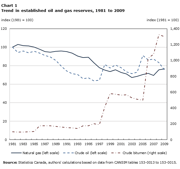
The established reserve of oil and gas in Canada has experienced a large compositional shift towards crude bitumen. As shown in Chart 1, from 1981 to 2009, the established reserve trended down slightly for both natural gas and crude oil. It dropped by about 25% for both natural gas and crude oil over the whole sample period. At the same time, the established reserve of crude bitumen increased dramatically, especially during the periods from 1997 to 1999 and after 2005. It increased by more than 12 times, or about 9.6% per year on average.

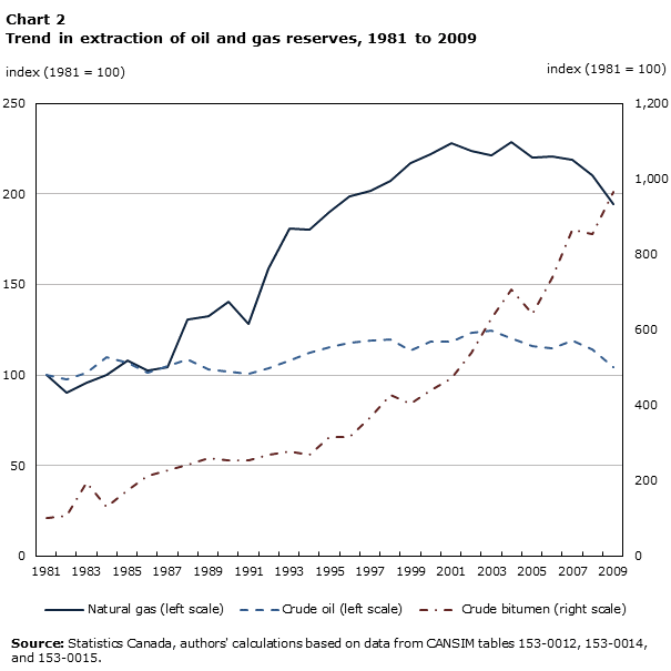
Unlike the pattern of the established reserve over time, the extraction of all three oil and gas resources has increased, although at quite different paces (Chart 2). From 1981 to 2009, extraction grew by about 2.4% per year for natural gas, by 0.1% per year for crude oil, and by 8.4% per year for crude bitumen.

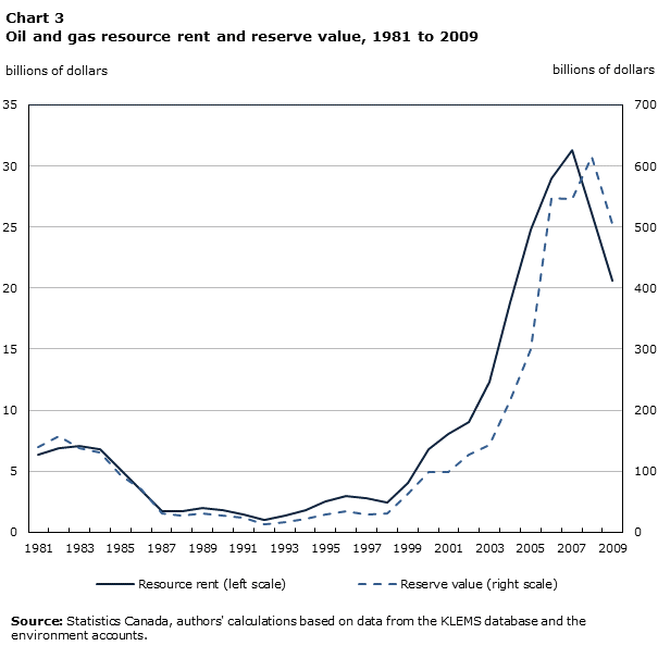
3.2 Resource rent and reserve value

Chart 3 presents the estimated value of oil and gas reserves and the resource rent from the extraction of oil and gas from 1981 to 2009. As shown, the patterns of the reserve value and resource rent, over time, are quite close to each other. Both stayed low and stagnant before 1999, and then grew rapidly thereafter. The annual resource rent declined by 2.5% per year over the 1981-to-1999 period and by 17.7% per year over the 1999-to-2009 period. The corresponding growth rates for the reserve value were -4.2% and 22.9% per year for the two periods, respectively.

3.3 Natural capital stock and natural capital input

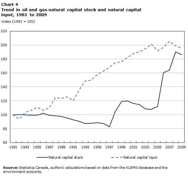
The natural capital input in this industry trended up steadily without major interruptions (Chart 4). It grew by 2.4% per year on average from 1981 to 2009. At the same time, the pattern of the natural capital stock, over time, is quite different from that of the natural capital input. The natural capital stock trended down gradually and dropped by about 17% before 1997, reflecting the down-trending movements in natural gas and crude oil reserves. After 1997, the natural capital stock exhibited a pattern, over time, similar to that of crude bitumen. It increased largely from 1997 to 1999 and after 2005, and decreased moderately from 2000 to 2005.

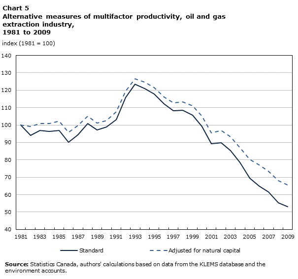
3.4 Multifactor productivity growth

In the growth accounting framework, adding natural capital has no impact on either output (value-added) growth or the contribution of labour input. However, the income share and, hence, the contribution of produced capital input will be reduced; as a result, MFP growth would be impacted if the produced capital input and the natural capital input grew at different paces.

As shown in Chart 5, MFP growth in oil and gas extraction was positive before 1993, and became largely negative after 1993. Note that adding natural capital in the growth accounting framework has little impact on the pattern of MFP growth over time. After adjusting for natural capital, annual MFP growth increases from 1.8% to 2.0% before 1993, and from -5.1% to -4.0%, after 1993.

Overall, by including subsoil resources, MFP declines by 1.5% per year over the 1981-to-2009 period, compared to a 2.2% decline without including these resources.

3.5 Natural capital contribution to value-added growth

The contribution of the natural capital input to the industry value-added growth is moderate in oil and gas extraction. From 1981 to 2009, the log growth of value-added in oil and gas extraction was about 2.3% per year, of which about 0.3 percentage points per year or 15% came from the growth in the natural capital input (Table 1).

4 Conclusion

To recognize subsoil energy and mineral resources as a capital input into the production process, this paper presents a growth accounting framework that allows the derivation of measures on natural capital stock and natural capital input in the mining industries and provides a better understanding of contribution of natural capital to economic growth and the impact of adding natural capital on productivity measurement.

The empirical results suggest a significant contribution of natural capital to the real value-added economic growth in the Canadian oil and gas extraction. However, the impact of adding natural capital in the growth accounting on the measured MFP growth changes over time. It is small before 1993 and becomes larger thereafter.

5 Appendix

References

Baldwin, J. R., and W. Gu. 2007. Multifactor Productivity in Canada: An Evaluation of Alternative Methods of Estimating Capital Services. The Canadian Productivity Review, no. 9, Statistics Canada Catalogue no. 15-206-X. Ottawa: Statistics Canada.

Brandt, N., P. Schreyer, and V. Zipperer. 2013. Productivity Measurement with Natural Capital. Economics Department, Organisation for Economic Co-operation and Development, Working Paper no. 1092. Paris: OECD.

Christensen, L.R., and D.W. Jorgenson. 1969. “The measurement of U.S. real capital input, 1929–1967.” Review of Income and Wealth 15: 293–320.

European Commission, International  Monetary Fund, Organisation for Economic Co-operation and Development, United Nations, and World Bank. 2009. System of National Accounts 2008. New York: United Nations.

Hotelling, H. 1931. “The economics of exhaustible resources.” Journal of Political Economy, 39 (2): 131–175.

Kendrick, J.W. 1976. The Formation and Stocks of Total Capital. New York: National Bureau of Economic Research.

Kronenberg, T. 2008. “Should we worry about the failure of the Hotelling rule?” Journal of Economic Surveys 22 (4): 774–793.

Livernois, J. 2009. “On the empirical significance of the Hotelling rule.” Review of Environmental Economics and Policy 3 (1): 22–41.

Miller, M.H., and C.W. Upton. 1985. “A test of the Hotelling valuation principle.” Journal of Political Economy  93 (1): 1–25.

Solow, R.M. 1974. “The economics of resources or the resources of economics.” The American Economic Review  64 (2): 1–14.

Statistics Canada. 2006. Concepts, Sources and Methods of the Canadian System of Environmental and Resource Accounts. Environment Accounts and Statistics Division, System of National Accounts. Statistics Canada Catalogue no. 16-505-G. Ottawa: Statistics Canada.

United Nations, European Commission, Food and Agriculture Organization of the United Nations, International Monetary Fund, Organisation for Economic Co-operation and Development, and World Bank. 2014. System of Environmental-Economic Accounting 2012: Central Framework. New York: United Nations.

Veldhuizen, E., M. de Haan, M. Tanriseven, and M. van Rooijen-Hoesten. 2012. The Dutch Growth Accounts: Measuring Productivity With Non-Zero Profits. Paper presented at the 32nd General Conference of the International Association for Research in Income and Wealth, Boston, August 5–11.

About Analytical Studies

The Analytical Studies Branch Research Paper Series provides for the circulation, on a pre-publication basis, of research conducted by Analytical Studies Branch staff, visiting fellows, and academic associates. The Analytical Studies Branch Research Paper Series is intended to stimulate discussion on a variety of topics, including labour, business firm dynamics, pensions, agriculture, mortality, language, immigration, and statistical computing and simulation. Readers of the series are encouraged to contact the authors with their comments and suggestions.

Papers in the series are distributed to research institutes, and specialty libraries. These papers can be accessed for free at www.statcan.gc.ca.

Acknowledgements

The authors would like to thank John Baldwin, Wulong Gu, Michael Wright of Statistics Canada; Pierre-Alain Pionnier of the OECD; Michael Smedes of the Australian Bureau of Statistics; Vernon Topp of the Australian Productivity Commission; Erik Veldhuizen of Statistics Netherlands; and Carl Obst of the London Group for their valuable comments and suggestions. Thanks also to  participants of the 2013 CANSEE (Canadian Society for Ecological Economics) conference at York University, Toronto; and 2014 NAPW (North American Productivity Workshop) VIII Conference at Ottawa/Gatineau, for helpful discussions. Any errors are those of the authors.