Provincial Convergence and Divergence in Canada, 1926 to 2011

View the most recent version.

Archived Content

Information identified as archived is provided for reference, research or recordkeeping purposes. It is not subject to the Government of Canada Web Standards and has not been altered or updated since it was archived. Please "contact us" to request a format other than those available.

Archived

This page has been archived on the Web.

by W. Mark Brown and Ryan Macdonald

Skip to text

• Abstract
• Executive Summary
• 1 Introduction
• 2 Data
• 3 Convergence
• 4 Provincial groupings
• 5 Conditional convergence
• 6 Conclusion
• 7 Appendix

Text begins

Abstract

This paper examines provincial convergence of per capita household disposable income in Canada over the 85 years from 1926 to 2011. The paper finds that convergence has not followed a smooth, continuous process, but rather, a series of pulses involving both convergent and divergent phases. While provincial incomes tended to converge, there were also periods when incomes diverged corresponding to large external shocks: 1) the Great Depression from the late 1920s to the mid-1930s; 2) the postwar transition from the mid-1940s to the early 1950s; 3) the oil price shocks from 1973 to the mid-1980s; and 4) beginning in 1996, a period that covers the resource boom of the 2000s.

The analysis also suggests that one group of provinces has generally been converging toward a common income level, while the second has followed its own growth path. The second group, composed of Alberta and Saskatchewan, and after 1996, Newfoundland and Labrador, largely accounted for the periods of divergence, especially those coinciding with the oil shocks of the 1970s and 1980s and the resource boom of the 2000s.

Keywords: Economic growth, convergence, personal income, household income.

Executive summary

This analysis examines provincial income convergence in Canada from 1926 to 2011 using National Accounts-based estimates of per capita household disposable income. Household disposable income is the income available for consumption and saving, and is, therefore, closely aligned with material well-being.

The paper presents two major findings. First, convergence was not a smooth, continuous process. Rather, periods of convergence were punctuated by periods of divergence. Second, based on their growth relative to the Canadian average, provinces can be divided into those that appear to be converging toward a common income level and those that are following their own paths.

Convergence is a long-run tendency for income levels between economies to become more similar. In its most literal sense, convergence implies that all provincial per capita disposable incomes across Canada will eventually reach the same level. Less exacting forms of convergence allow for differences in per capita income levels due to structural differences across provinces. Factors such as resource endowments, urbanization, human capital, and industry structure are believed to be sources of such differences.

From 1926 to 2011, the average annual rate of convergence across Canada was 1.3%. This can be interpreted as the rate at which differences in provincial per capita income levels were removed. (At 1.3% a year, it would take 53 years to remove half the difference between provincial per capita income levels.) This estimate excludes Newfoundland and Labrador, which did not join Confederation until 1949, and is below most rates reported in the literature. An estimate for the 1949-to-2011 period that includes Newfoundland and Labrador yields an annual unconditional convergence rate of 2.3%, which is similar to other estimates.

During periods of convergence, the annual rate ranged from 3.3% to 6.3%. For the periods of divergence, coefficient values are typically smaller, and not statistically significant. The only period with a negative coefficient was 1945 to 1951.

The average rate of convergence is higher when the different patterns that were followed by Alberta and Saskatchewan are taken into account in the regression analysis. In most convergent periods, as well as in long-run estimates, adjusting for Alberta and Saskatchewan increases the rate. For the entire 1926-to-2011 period, the estimate rises from 1.3% to 1.9%; for the 1949-to-2011 period, it increases from 2.4% to 3.6%.

The periods of divergence coincided with some of the largest external shocks that have affected the Canadian economy, but they did not correlate with business cycles. In particular, the U.S. recessions of the 1950s, 1960s and 1990s were not associated with divergence. Rather, the events that produce divergence are related to relative price shocks that have an asymmetric effect, often boosting demand in one region while reducing demand in others. The Great Depression brought swings in relative prices, as did the removal of price controls after the Second World War, the oil shocks of the 1970s, and the resource boom in the first decade of the 21st century.

Convergence of per capita household disposable income toward a similar level is apparent for most provinces. However, this was not the case for Alberta and Saskatchewan, whose growth paths moved in tandem over time, often across the distribution of relative provincial per capita incomes. They reached lows during the 1930s (sixth place for Alberta, tenth for Saskatchewan), but by the 2000s, both provinces were ranked at the top of the income distribution (first for Alberta, second for Saskatchewan). Their shared path has been an important driver of the divergence–convergence dynamic, and since 1996, they have been joined by Newfoundland and Labrador.

1 Introduction

Numerous studies of Canadian income growth have found strong evidence of convergence across provinces (e.g., DeJuan and Tomljanovich 2005; Gunderson 1996; Coulombe and Lee 1995). Predominantly focusing on the 1950-to-2000 period, and often using different time spans and income measures, these studies show that human capital is an important source of convergence (Coulombe 2011; Coulombe and Tremblay 1998; Coulombe 2000, 2003, 2006). They also demonstrate that natural resource endowments affect income allocation (Lee 1996; Afxentiou and Serletis 1998), that the economic structure associated with urbanization is important in concentrating human capital (Coulombe 2000, 2003, 2006), and that the Canadian fiscal transfer system can affect convergent economic forces, for example, by reducing interprovincial reallocation of labour (Coulombe and Day 1999; Kaufman, Swagel and Dunaway 2003; Darku 2011).

Although previous studies reported a tendency toward convergence, recent data show that provincial incomes diverged after 1996. This runs against expectations, because no substantive changes occurred in the standard variables used to explain income level differences across provinces during that period. This paper asks which provinces stand out as causing the divergence, and by extending the analysis back to 1926, seeks to determine whether the recent period of divergence is unique.

Three major findings emerge from this analysis. The first is a tendency for short-run dynamics to temporarily supplant long-run trends. Convergence occurs slowly (1.5% to 3.0% annually; Sala-i-Martin 1996a), and as a result, macro-economic shocks can overwhelm the process in the short run. However, it takes more than an exogenous demand shock to produce a period of divergence. Divergent periods in Canada do not have a one-to-one correspondence with events such as recessions in the United States. They do, however, coincide with periods of significant relative price changes, such as the Great Depression, the oil shocks of the 1970s, and the commodity boom of the 2000s.

The second notable finding is that specific provinces may have a long-run steady-state equilibrium that differs considerably from the other provinces. Previous analyses took this into account by including additional covariates. The present study, which analyzes provinces individually relative to the Canadian average, shows that Alberta and Saskatchewan moved around the distribution of provinces, and that they moved in tandem through time. Using an extended time series that includes the commodity boom of the 2000s, this analysis demonstrates that these provinces followed an upward trajectory relative to the Canadian average, but also one that oscillated across periods. While their joint trajectory sometimes works toward convergence and sometimes against it, over the last 85 years these provinces have been moving toward long-run equilibriums that differ from those of other provinces.

The third major finding is that the long-run equilibrium itself evolves through time. Examining the paths of provinces individually reveals instances where development of a new industry changed the steady state. In Alberta, Saskatchewan, and Newfoundland and Labrador, the hydrocarbon industries stand out as likely sources of change in the steady-state equilibrium. The increased importance of oil and gas extraction in Alberta and Saskatchewan in the 1970s appears to have permanently altered their relative growth paths. Similarly, before 1997, Newfoundland and Labrador’s income growth was in line with that of the other Atlantic Provinces. After 1996, when offshore production began, Newfoundland and Labrador’s income growth relative to the Canadian average changed to match that of Alberta and Saskatchewan, implying that the steady-state value changed.

The remainder of this report is structured as follows. Section 2 describes the data used. Section 3 examines classical convergence measures. Section 4 moves beyond the classical structure normally employed in convergence studies to illustrate the heterogeneity of the convergence process across provinces. Section 5 extends the classical convergence measures to take into account the differing patterns of convergence, or lack thereof, across provinces. Section 6 concludes.

2 Data^Note 1

This analysis uses per capita household disposable income to study the convergence process, primarily because an 85-year time series is available for this measure. The long time span is valuable, as convergence typically occurs at around 2% annually^Note 2 (for example, Barro et al. 1991; Sala-i-Martin 1996b). As well, household disposable income is closely aligned with material well-being.^Note 3 It consists of wages, salaries, supplemental labour income, transfers from governments to persons, net of taxes paid, as well as dividends and interest payments. It incorporates the effect of the fiscal transfer system and investment income.

Constructing a long time series for household disposable income requires three data vintages from the Canadian System of National Accounts. A historical 1926-to-1986 vintage is used for the years from 1926 to 1960. A historical 1961-to-2010 vintage is used for 1961 to 2006, and a modern 2007-to-2011 vintage is used for the most recent period.

Because definitions and concepts vary across vintages, linking the data sources is a challenge. The historical vintages contain an amalgam of households, non-profit institutions serving households (NPISH) and unincorporated businesses (the self-employed). The modern vintage excludes the NPISH sector.^Note 4 Because the Provincial Economic Accounts do not calculate a set of sector accounts outside the household sector, it is not possible to approximate the previous aggregation as closely as desired. The data in this analysis link the modern household sector provincial incomes to an instrument composed of households and NPISH. This creates an inconsistency between the modern and historical data, which affects levels more than growth rates. The largest differences occur for Prince Edward Island.

To produce series with the least effect from revisions, the modern estimates are back-cast using the growth rates from the historical vintages. The linking procedure will affect the historical levels relative to published sources. However, the structure of historical growth rates is maintained, and the relative positions of all provinces are unchanged for the overlapping 2007-to-2010 period. Consequently, little change occurs in the information relevant for assessing convergence. Population data are from Statistics Canada’s CANSIM database. Data from tables 380-0043 and 051-0005 are combined to produce the long-run population estimates.

The nominal estimates of household disposable income by province are reported relative to the 10-province aggregate value of per capita income. This value is referred to as the average value of Canadian per capita income. To permit the long-run analysis, the influence of inflation on the purchasing power of income through time was accounted for by comparing each provincial estimate with the aggregate value. This is similar to the approach applied in studies of savings rates, which account for inflation by reporting estimates as a fraction of income.

As a robustness check, analytical measures are re-calculated using real income estimates where price indexes based on consumer price calculations for major cities are employed. The results are reported in the Appendix. Price indexes for the capital city of each province from three sources are linked. These indexes provide long-run indications of price growth. For 1971 to 2011, the data are from CANSIM table 326-0021. For 1940 to 1970, city Consumer Price Index (CPI) estimates are from series K23 of the historical statistics of Canada. Finally, for 1926 to 1939, the data source is Emery and Levitt (2002).

To construct the long-run city CPIs, growth rates are used to back-cast the indexes. For Prince Edward Island, the series from Charlottetown begins in 1974 in the modern data. The Historical Statistics of Canada do not include a Charlottetown series; the value for Saint John, New Brunswick, is used instead. For St. John’s, the price data begin in 1952, three years after Newfoundland and Labrador entered Confederation. An average of the growth rates from Saint John and Halifax is used to backcast the price index for St. John’s back to 1949.

3 Convergence

At the outset, it is useful to establish a number of stylized facts. Perhaps the most important is whether provincial per capita household disposable incomes have converged or diverged, and during which periods. Here, a measure of dispersion based on the range of the data is used to identify periods of income convergence and divergence. This simple measure complements the more commonly used sigma (standard deviation). Whereas sigma takes the entire income distribution into account, the range focuses on differences between the highest and lowest provincial per capita incomes.

Throughout the paper, provincial per capita incomes are measured relative to aggregate national per capita income. If unconditional convergence holds across provinces, the range of the data should diminish, presenting a triangular shape, as provincial income levels approach the common national value. Conversely, if conditional convergence prevails, provinces should approach the same growth rate through time, but at different income levels. This would result in a distribution over time that would eventually display a quasi-rectangular (trapezoidal) shape.

Chart 1 displays the range of per capita provincial estimates relative to the Canadian average. The bottom of each line is the lowest provincial per capita income relative to the national average for each year; the top is the highest; and the distance between the lines covers the range of data. The wider the range, the more dispersed is provincial per capita income. The section covering the 1950-to-2000 period encompasses the time spans used in most convergence studies. As Chart 1 shows, a triangular shape persisted over a long period, which suggests that unconditional convergence, or something close to it, occurred among provinces for much of the 1926-to-2011 period

Description for chart 1

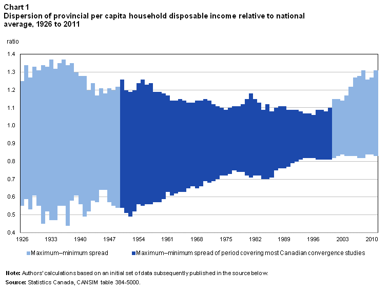
Chart 1 also illustrates several other features of Canadian convergence. First, and foremost, it is not a smooth process. In four periods, divergence rather than convergence occurred in the range of the data: 1) from the late 1920s to the mid-1930s;^Note 5 2) from the mid-1940s to the early 1950s; 3) from the first oil shock in 1973 to the mid-1980s,^Note 6 when oil prices declined sharply; and 4) beginning in 1996 and continuing through the resource boom of the 2000s. The episodes of divergence coincided with some of the largest economic shocks of the 20th century, and appear as periods of divergence in other measures of dispersion. Aside from these four periods, convergence was the norm. The data suggest that convergence across Canadian provinces is better described as a pulsing rather than a continuous process. Nonetheless, since 1926, convergent forces outweighed divergent forces.^Note 7

The second feature apparent in Chart 1 is that convergence was asymmetric. More convergence occurred from the bottom up than from the top down. The lowest relative provincial per capita income—43.6% of the national average—occurred in 1937; by 2011, the corresponding figure was 84.3%, an increase of 40.7 percentage points. The highest relative provincial per capita income—136.0% of the national average―occurred in 1936; this fell to a low of 105.7% in 1996, a drop of 30.2 percentage points.

Third, divergence after 2000 was primarily due to above-average provincial per capita incomes rising rapidly. In the three other periods of divergence, divergence from below was more prevalent. In this respect, the divergence of the 2000s is unique.

Finally, through a combination of happenstance, data constraints and the dates at which research was published, most Canadian convergence studies focus on the years from 1950 to 2000, a period when convergence predominated across Canadian provinces.

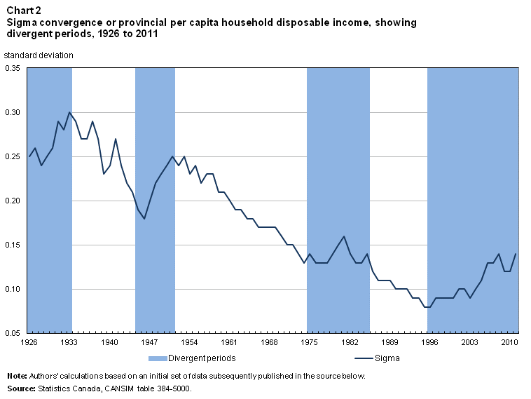
To confirm the pattern of convergence and divergence through time, Chart 2 uses sigma to measure dispersion.^Note 8 Sigma measures the dispersion of the distribution of provincial per capita incomes relative to the Canadian average. If all provinces are close to the average, then the sigma estimate is small while if provinces are father away from the Canadian average, then the estimate is larger. If the distribution is becoming more bunched through time, then the estimate of sigma will decline through time.

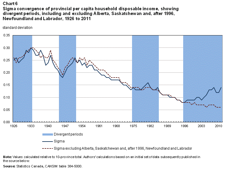
Chart 2 shows that the patterns in sigma estimates conform closely with the simpler, range-based measure from Chart 1. The shaded areas represent the periods of divergence identified above, and in each period, there was a tendency for the dispersion of provincial income to increase, or in the case of 1973 to 1986, to pause.

Description for chart 2

3.1 Unconditional convergence

The assumption underlying unconditional convergence stems from the Solow growth model (Solow 1956). Unconditional convergence posits that all provinces will eventually reach a common per capita income level (for example, Sala-i-Martin 1996a). At first, it appears that this occurred during much of the period since 1926.

A common method of estimating convergence relates initial income levels to subsequent income growth rates (Barro and Sala-i-Martin 1995; Sala-i-Martin1996a). Typically, the following equation is used:^Note 9

$$\left(\frac{1}{T-t}\right)\left[\left(\raisebox{1ex}{$\ln (y_{i,T})$}\!\left/ \!\raisebox{-1ex}{$\ln (y_{i,t})$}\right.\right)\right]=\alpha -\left[1-e^{\left(-\beta (T-t)\right)}\right]\times \ln (y_{i,t})\times \left(\frac{1}{T-t}\right). (1)$$

Equation (1) relates the speed at which provincial per capita incomes grow to their initial levels. $y_{i,T}$ is relative per capita income in province $i$ at the end of the period $(T)$, and $y_{i,t}$ is income in province $i$ at the start of the period $(t)$. As long as the speed of convergence $(\beta )$ lies between 0 and 1, the incomes in question converge toward a common steady state. For the study period, estimates of the speed of convergence are calculated from Equation (1) using non-linear least squares (Table 1). Provincial per capita incomes are measured relative to the Canadian average. Estimates for $\beta$ are reported for the entire period, and for the specific episodes of convergence and divergence described above. The number of provinces used for analysis increases when Newfoundland and Labrador enter Confederation in 1949.

For the periods of convergence, 1936 to 1945 corresponds to the recovery from the Great Depression; 1951 to 1973, the ‘golden age’ of rising real income. For the periods of divergence, 1926 to 1936 corresponds to the Great Depression; 1945 to 1951, the transition from war-time to peace-time production; 1973 to 1986, the period of high energy prices brought about by the first and second oil shocks; and 1996 to 2011, the commodity boom of the early 21st century.

The regression estimates show a statistically significant annual rate of convergence of 1.3% for the entire 1926-to-2011 period. Although this is lower than estimates reported in some of the Canadian convergence literature, the estimate of 2.3% for the 1949-to-2011 period is of the same magnitude as those in other studies (Sala-i-Martin 1996b; Coulombe and Lee 1995).

The estimates for convergent periods are significant at the 5% nominal level, and have coefficient values ranging from 3.3% to 6.3% per annum. For the divergent periods, the coefficient values are smaller, and are not statistically significant. The only period with a negative coefficient spans 1945 to 1951. As we demonstrate in the next section, this reflects specific provinces diverging while the others continued to converge. As a result, the signal for convergence in the data becomes weaker, and regression techniques based on Equation (1) are not able to account for this.

4 Provincial groupings

The model that underlies unconditional convergence appears to have some explanatory power. However, differences across provinces in savings rates, urbanization and industrial structures have been shown to affect provincial per capita income levels (Lee 1996; Coulombe and Tremblay 1998; Coulombe 2000, 2003; Kaufman, Swagel and Dunaway 2003). Moreover, the intermittent pauses in the convergence process and the substantial divergence in the late 1990s suggest that some provinces may react differently to economic shocks. Therefore, it is useful as a prelude to, and justification for, the conditional convergence analysis that follows to ask whether specific provinces, or groups of provinces, show evidence that they are moving to different steady states or that their steady-state equilibriums have changed over time.

4.1 Aberrant observations, Alberta and Saskatchewan

One way to identify provinces that are behaving differently is to determine if they qualify as aberrant observations-that is, data points that do not align with the majority of results (Rousseeuw and Leroy 2003). Identifying aberrant observations can be challenging, but in the case of provincial convergence in per capita household income, complex algorithms are not necessary. A graphic presentation of the relationship posited by the unconditional convergence model's structure is sufficient. Chart 3 plots the initial value (1926) of per capita household disposable income in each province relative to the Canadian average (x-axis) against the average growth rate of per capita household disposable income in each province relative to the Canadian average (y-axis) from 1926 to 2011. The squares represent Alberta and Saskatchewan; the diamonds represent the other provinces (excluding Newfoundland and Labrador). Superimposed on the scatter plot are regression lines from an equation that relates average growth rates to the log of the initial value:

$${\overline{\dot{y}}}_{i,1926-2011}=\alpha +\beta \ln (y_{,i1926})+{\epsilon }_i$$

The linear relationship rather than the non-linear convergence model is used to highlight the aberrant provinces. The solid line represents the line of best fit including all provinces; the dashed line represents the line of best fit excluding Alberta and Saskatchewan. The solid line that includes all provinces creates larger errors and passes through mostly empty space. The dashed line that excludes Alberta and Saskatchewan passes through most data points. The implication is that Alberta and Saskatchewan behave differently than the other provinces, and that they influence regression results.

Description for chart 3

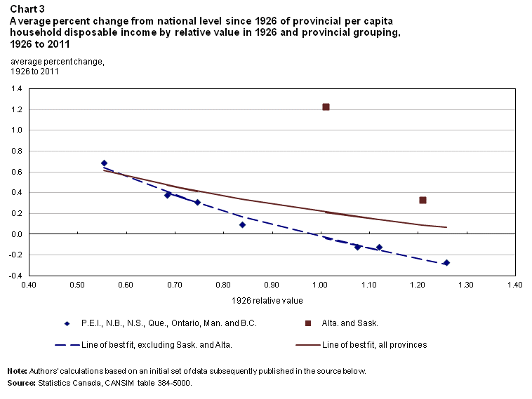
The same exercise is performed for the 1949-to-2011 period that includes Newfoundland and Labrador, as well as for each period of convergence and divergence identified above. Residuals for Alberta and Saskatchewan are calculated based on the fitted values from the line of best fit from the restricted sample (i.e., Alberta and Saskatchewan are omitted from the estimation, but their predicted values using the regression coefficients are compared with their actual values to calculate a residual). In both long-run periods (1926 to 2011 and 1949 to 2011), the residuals for Alberta and Saskatchewan are noticeably larger than the residuals for the other provinces (Table 2). The pattern is the same in the divergent periods—Alberta and Saskatchewan are noticeably off the regression plane and create large errors.

In the periods of convergence, Alberta and Saskatchewan move down to the regression plane of the other provinces, and produce residuals similar to those of the other provinces. The exception is the 1936-to-1945 period, during which per capita income in Alberta and Saskatchewan rose more rapidly than the national average, but from a starting point below it. Consequently, their outsized influence biased the results toward faster convergence rather than toward divergence, and largely explains the high rate of convergence in the 1936-to-1945 period in Table 1.

The conclusion to be drawn from the residuals is that per capita income in Alberta and Saskatchewan have fluctuated in a way that differed from the other provinces, which implies that they followed a different growth process. This implication is examined throughout the remainder of this analysis, and henceforth, Alberta and Saskatchewan are designated own-growth-path (OGP) provinces.^Note 10

The notion that the OGP provinces follow a different path is strengthened when their average per capita household income is contrasted with that of the non-OGP provinces. OGP per capita income is composed of Alberta, which tended to be above the national average, and Saskatchewan, which was often below the national average. Because Alberta and Saskatchewan have co-integrated growth paths (see co-integration tests below), the relative performance of their combined average is an appropriate representation of how their per capita household income behaved over time relative to the national average, even if the Alberta values tended to dominate the relative level.

Relative to the national average, the OGP provinces alternated between falling behind and surging ahead (Chart 4). During the Great Depression and the ‘golden age’ of rising real income (1951 to 1973), agricultural prices (the major resource output of the OGP provinces at that time) tended to decline relative to prices of manufactured goods and services. As a result, per capita income growth of the OGP provinces generally lagged behind that of the rest of the country and fell below the national average. The 1973 oil shock reversed this tendency, and even from 1987 to 2000, when real oil prices declined, per capita household income in the OGP provinces rose at an above-average rate. The increase in oil prices after 2000 accelerated this income growth relative to the rest of the country.

Description for chart 4

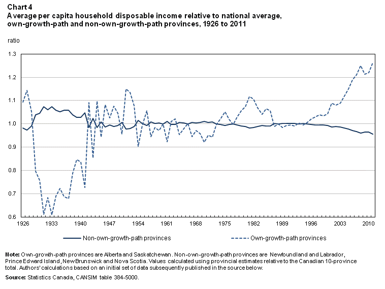
The early 1970s marked a turning point at which the industrial composition of the OGP provinces had shifted enough toward hydrocarbon production that events affecting these industries became significant for the overall provincial economy. Although there had been exploration activity in the OGP provinces during and before the Second World War, the hydrocarbon industry did not progress substantially until the discovery of oil in Leduc, Alberta, in 1947.

During this development phase, relative per capita income in the OGP provinces fell. Trends in per capita household income in the OGP provinces then followed the dynamics of oil prices through the first oil shock of the early 1970s, the second oil shock in 1979, and the eventual collapse of oil prices in 1986. After 1986, rather than declining, per capita income in the OGP provinces rose modestly relative to the national average, and after 2000, rose above it as oil prices increased. This dynamic illustrates how a shift in the use of the resource base of the OGP provinces translated into a long-term change in the relative behaviour of per capita income. It foreshadowed events that would occur in Newfoundland and Labrador.

4.2 Economic evolution, Newfoundland and Labrador

In light of the experience of Alberta and Saskatchewan, the question is whether per capita household income in Newfoundland and Labrador also responded when oil and gas production started in this province in the mid-1990s. Co-integration tests are used to determine if trends in Newfoundland and Labrador became similar to those in Alberta and Saskatchewan. In addition, the nature of the co-integrating relationship implied by the OGP aggregation of Alberta and Saskatchewan is formalized.

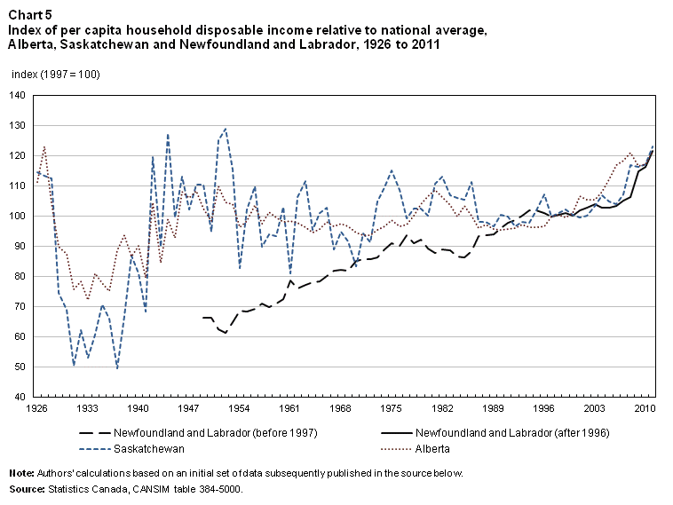
Per capita household income in Alberta, Saskatchewan, and Newfoundland and Labrador relative to the national average is converted into an index with a base year of 1997, the year when oil and gas production began in Newfoundland and Labrador. Throughout most of the 1926-to-2011 period, Saskatchewan’s income level relative to that of Canada followed the same pattern as Alberta’s, but with greater variance. A gap emerged between the two series in the 1930s, but it disappeared after the Second World War (Chart 5). After 1997, Newfoundland and Labrador followed a pattern almost identical to Saskatchewan with Newfoundland and Labrador’s per capita disposable income rising by 21.6% relative to the Canadian value between 1997 and 2011. The rise for Alberta over the same time period was 21.2% while for Saskatchewan it was 23.0%.

To test for co-integration, Johansen’s test using no deterministic trends is applied to pairs of provincial relative per capita income indexes. The results test the null hypothesis of no co-integration (Table 3). Tests are reported for two periods: 1926 to 2011 and 1997 to 2011. The 1926-to-2011 period, which pertains only to Saskatchewan and Alberta, presents the best results because the data cover a long time span, and are, therefore, more likely to reflect the influence of common factors on these provinces. The estimating equation for the longer period includes an exogenous indicator variable for the years from 1929 to 1942 in order to capture the relatively larger impact of the Great Depression on Saskatchewan. The results for the much shorter 1997-to-2011 period are less robust, owing to the relative lack of data.

For 1926 to 2011, the hypothesis of no co-integration between Saskatchewan and Alberta is rejected. For 1997 to 2011, the results are more ambiguous. The trace and max-eigenvalue tests continue to suggest co-integration between Alberta and Saskatchewan, but only the trace statistic suggests co-integration between Alberta and Newfoundland and Labrador or between Saskatchewan and Newfoundland and Labrador. The max-eigenvalue statistic fails to reject the null hypotheses of no co-integrating vectors. Overall, the assumption that Alberta and Saskatchewan are affected by a common factor is supported by the data. Support is weaker for the relationship between the Prairie provinces and Newfoundland and Labrador, but evidence supports the hypothesis that Newfoundland and Labrador co-integrated with Saskatchewan after 1996.

Description for chart 5

5 Conditional convergence

The OGP provinces followed a similar path through time that moved across the distribution of the converging provinces. They appear to be converging to a different steady state from the other provinces, and are the source of the observed divergence—convergence dynamic. That being the case, it is natural to ask what the convergence measures would be like if the effect of these provinces were taken into account.

Unconditional convergence relies on assumptions about similarities in savings rates, technological progress, and population growth across provinces. An alternative version of convergence—conditional convergence—posits that provinces have the same rate of convergence, but that there may be differences between their long-run growth rates due to differences in the structure of provincial economies. The standard model for convergence can be augmented to include explanatory variables; that is, convergence rates are estimated “conditional” on these additional factors.

As a starting point, Equation (1) is re-estimated including an indicator variable (delta) for the OGP provinces (Equation [2]). This indicator represents differences in provincial resource endowments that, in turn, create differences in long-run, steady state growth rates. Here we treat Newfoundland and Labrador as though it switches from the non-OGP group to the OGP group in the mid-1990s. For the 1949-to-2011 and 1996-to-2011 periods, a separate model is estimated that includes Newfoundland and Labrador in an expanded indicator variable.

$$\left(\frac{1}{T-t}\right)\left[\left(\raisebox{1ex}{$\ln (y_{i,T})$}\!\left/ \!\raisebox{-1ex}{$\ln (y_{i,t})$}\right.\right)\right]=\alpha -\left[1-e^{\left(-\beta (T-t)\right)}\right]\times \ln (y_{i,t})\times \left(\frac{1}{T-t}\right)+\delta I_{OGP} (2)$$

The results are presented in Table 4. For the 1926-to-2011 period, adjusting for the indicator variable accelerates the estimated rate of convergence. For the period after 1949, which includes Newfoundland and Labrador, the annual rate of convergence rises to 3.6% when only the effect of the OGP provinces is taken into account. The rate of convergence falls to 2.1% when Newfoundland and Labrador is treated as an OGP province.

For the three periods of convergence, the conditional convergence rate is slower than the unconditional rate: 4.1% versus 6.3% for 1936 to 1945; 2.8% versus 3.3% for 1951 to 1973; and 4.0% versus 4.4% for 1986 to 1996. For the periods of divergence (except 1926 to 1936), the estimates of the speed of conditional convergence exceed the estimates of unconditional convergence. For the 1945-to-1951 period, conditional convergence is estimated at -0.9%, compared with -1.5% for unconditional convergence. The 1973-to-1986 period does not have as large a change. However, for the 1996-to-2011 period, when the OGP indicators are included, conditional convergence is estimated at 5.3%, compared with 1.4% for unconditional convergence.

In the case of sigma, there are differences each year due to differences in the sample used to calculate the dispersion (Chart 6). Throughout most of the time series, the dispersion estimate based on all 10 provinces (Sigma) is higher than the estimate based on the converging provinces (Sigma-exclOGP). This is because the OGP provinces were often the highest per-capita-income jurisdictions. There is less variability in the Sigma-exclOGP time series in the 1920s and 1930s, and similar movements in Sigma and Sigma-exclOGP between the 1930s and the first oil shock in 1973. However, after 1996, Sigma-exclOGP continues to fall for the convergent provinces, while Sigma moves in the opposite direction.

The regression results and the dispersion estimates provide complementary evidence that the behaviour of per capita household income of the OGP provinces differs from that of the converging provinces. When indicator variables are used to account for the OGP provinces, the speed of convergence accelerates. When the OGP provinces are excluded from the dispersion estimates, the signal for convergence has less noise, and periods of divergence in the latter half of the study period are mostly accounted for. Although the pause in convergence during the 1973-to-1986 period remains, divergence after 1996 is completely accounted for in the estimate of sigma. In fact, when the OGP and Newfoundland and Labrador are excluded, Sigma-exclOGP estimates show no divergence after 1996.

Description for chart 6

6 Conclusion

To some extent, the analysis of convergence of provincial household disposable income per capita is constrained by the small number of units (10) studied. Consequently, the use of more than one analytical technique yields a better understanding of the evolution of provincial per capita income. This study used cross-section regression techniques to provide inference, and a number of features of the distribution of provincial per capita household income through time were examined. In the future, development of a panel dataset with the necessary covariates to study convergence would provide greater insight.

Since 1926, per capita household income converged across most provinces. However, the process was not smooth, and in some periods, provincial per capita incomes diverged. Specifically, divergence occurred during the Great Depression, the return to peacetime production after the Second World War, the years from 1973 to 1986 when the price of energy products was elevated, and the commodity boom of the 2000s.

The periods of divergence coincided with major external shocks that affected the Canadian economy over the last 85 years, but they did not correspond to business cycles. In particular, the recessions of the 1950s, 1960s and the 1990s were not associated with divergence. The major external shocks had an asymmetrical effect, often boosting demand in one region and simultaneously suppressing demand in others, and thereby creating divergence in provincial per capita household income. The Great Depression was associated with swings in relative prices, as was the removal of price controls after the Second World War, the oil shocks of the 1970s, and the resource boom during the first decade of the 21st century.

Nonetheless, among most provinces, per capita household income converged. By contrast, household income in Alberta and Saskatchewan did not converge toward the national level, but instead, moved around the income distribution during periods of economic shocks, reaching lows during the 1930s (6th place for Alberta,10th for Saskatchewan) and highs during the 2000s (1st place for Alberta, 2nd for Saskatchewan). Their paths over time were similar, and were primarily responsible for the divergence–convergence dynamic since the end of the Second World War. After Newfoundland and Labrador joined Confederation in 1949, household disposable income in the province rose toward to the national average until 1996. Thereafter, the trend in Newfoundland and Labrador became similar to Saskatchewan’s, moving up across the provincial income distribution.

Accounting for the influence of Alberta, Saskatchewan, and after 1996, Newfoundland and Labrador, accelerates the estimated rate of convergence and yields results that indicate continued convergence after 1996. Thus, much of the divergence in provincial per capita household income in Canada, after the Second World War was attributable to these three provinces.

7 Appendix

7.1 Provincial rankings

A complementary method of illustrating the different provincial experiences is to rank provincial per capita incomes (Table 5). Alberta and Saskatchewan had most of the changes in ranking during the 1926-to-2011 period. Alberta moved between 1st and 6th position, and Saskatchewan, between 2nd and 10th. Through the first decade of the 2000s, Newfoundland and Labrador rose from 10th to 5th position.

British Columbia and Ontario declined in the rankings as Alberta and Saskatchewan rose. Manitoba consistently ranked fourth, but recently, dropped to eighth. The provinces converging from below tended to have a stable ranking.

Although the provincial rankings are informative, the magnitude of relative changes is important for putting shifts in relative position in context (Table 6). Early in the time series, when per capita household incomes were more dispersed, moving between ranks meant a greater change in relative income. Later, and especially during the 2000s when incomes were more closely grouped, a change in rank did not necessarily signal a substantial change in relative income.

During the Great Depression, Alberta and Saskatchewan experienced large jumps across the ranking that reflected 55- and 56-percentage-point declines in their relative per capita household disposable income. These changes had the effect, all else being equal, of elevating other provinces. The shifts after 2000 were associated with much smaller changes. Saskatchewan and Newfoundland and Labrador experienced the largest changes in rank, rising from 7th to 2nd, and from 10th to 5th, respectively. These shifts were accompanied by 20- and 17-percentage-point changes in their relative incomes, less than half the magnitude of the change in the 1930s. (Alberta did not change rank after 2000—it remained first—but its relative income rose by 22 percentage points.)

Among the provinces that declined in the rankings between 2000 and 2011, the largest drops were Quebec (from fifth to ninth) and Manitoba (from fourth to eighth). However, the magnitude of the changes relative to the national average was 2 percentage points for Quebec and 1 percentage point for Manitoba. So while the rank order changed, the magnitude of the shift was minimal.

7.2 Robustness check

To this point, nominal data were used to examine convergence. To assess the robustness of the analysis, deflated estimates were also employed. City-CPI series were used to deflate the provincial measures of per capita household income. The relative values for the provinces were then re-calculated. The 10 province values for Canada-wide per capita income use the All-items CPI for a deflator. The base year for all series was 2002, in which purchasing power across provinces is assumed to be equal.

When deflated data are used, the results are broadly unchanged. Chart 7 shows the range of values for relative incomes, and the path of the divergent provinces. Chart 8 shows estimates of sigma including and excluding Alberta and Saskatchewan. In both instances, the fundamental pattern of the data persists.

Description for chart 7

Description for chart 8

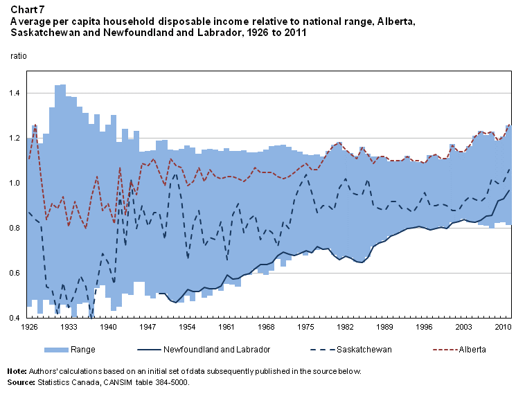
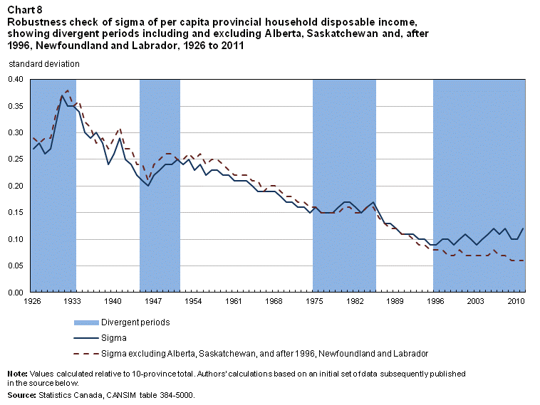
Alberta and Saskatchewan continue to diverge from the other provinces—estimates of sigma show convergence in provincial per capita household incomes when they are excluded, but divergence when they are included. The tendency for Alberta and Saskatchewan to follow their own path remains, and is more stable around a long-term upward trajectory than the nominal data suggest.

The largest difference that emerges when the deflated data are used is in the spread. In the nominal data, there is an increase in the spread from above and below during the 1926-to-1936 period and during the 1945-to-1951 period, whereas in the deflated data, the increase in the spread from below is reduced. For the Depression years of the 1930s, there is a larger increase in dispersion above the average, but in the 1945-to-1951 period, there is little noticeable change. Nevertheless, during the 1926-to-1936 period and the 1945-to-1951 period, an increase in estimates of sigma remains. In other words, when deflated data are employed, the earlier period continues to show an increase in dispersion around the same points in time, but not necessarily as a result of movements at the top and bottom of the distribution.

Similarly, Table 7 shows the results from the conditional convergence regressions. The deflated data yield estimates of similar magnitude, and a similar pattern of accelerated periods of convergence punctuated by pauses.

Notes