
Dealing with small sample sizes, rotation group bias and discontinuities in a rotating panel design 2. Design of the Dutch Labour Force Survey
The objective of the Dutch LFS is to provide reliable information about the Dutch labour force. Each month a stratified two-stage cluster design of addresses is drawn. Strata are formed by geographical regions. Municipalities are considered as primary and addresses as secondary sampling units. All households residing at an address, up to a maximum of three, are included in the sample. Different subpopulations are oversampled to improve the accuracy of the official releases, for example, addresses where people live who are formally registered at the employment office, and subpopulations with low response rates.
Before 2000, the LFS was designed as a cross-sectional survey. Since October 1999, the LFS has been conducted as a rotating panel design. Until the redesign in 2010, data in the first panel were collected by means of computer assisted personal interviewing (CAPI). Respondents were re-interviewed four times at quarterly intervals by means of computer assisted telephone interviewing (CATI). During these re-interviews, a condensed questionnaire was used to establish changes in the labour market position of the respondents. The monthly gross sample size for the first panel averaged about 8,000 addresses commencing the moment that the LFS changed to a rotating panel design and gradually fell to about 6,500 addresses in 2012. The response rate is about 55% in the first panel and in the subsequent panels about 90% with respect to the responding households from the preceding panel.
The estimation procedure of the LFS starts with the GREG estimator. Inclusion probabilities reflect the sampling design and differences in response rates between geographic regions. The weighting scheme is based on a combination of different socio-demographic categorical variables. Key parameters of the LFS are the employed, unemployed and total labour force, which are defined as population totals. Another important parameter is the unemployment rate, which is defined as the ratio of the unemployed labour force to the total labour force.
Figure 2.1 illustrates the RGB for the unemployed labour force. The series of the GREG estimates of the first panel are compared with the average of the GREG estimates of the four subsequent panels. The GREG estimates for the unemployed labour force in the subsequent panels are systematically smaller than in the first panel. The RGB is a consequence of different non-sampling errors like selective non-response, panel attrition, mode-effects, effects due to differences between the CAPI questionnaire and the CATI questionnaire, and panel effects.
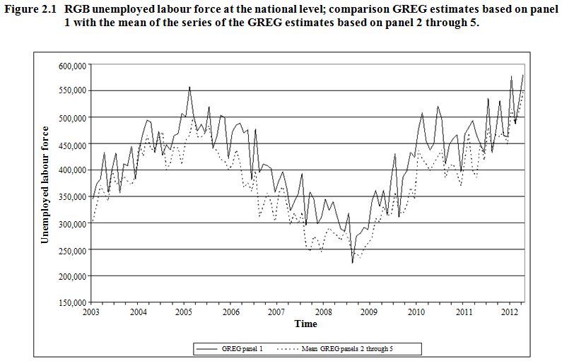
Description for Figure 2.1
This is a line chart. The horizontal axis is the time. The vertical axis is the unemployed labour force. There are 2 series in this graph: the GREG estimates based on panel 1 and the mean of the series of the GREG estimates based on panel 2 through 5. The data are in the following Table:
| Time | GREG panel 1 | Mean GREG panels 2 through 5 |
|---|---|---|
| Jan-03 | 345,022.53 | 303,292.89 |
| Feb-03 | 373,661.22 | 332,539.48 |
| Mar-03 | 383,517.25 | 370,716.15 |
| Apr-03 | 433,681.78 | 355,597.88 |
| May-03 | 357,097.78 | 341,464.13 |
| Jun-03 | 402,452.59 | 399,602.89 |
| Jul-03 | 431,846.44 | 373,892.09 |
| Aug-03 | 356,306.31 | 375,690.34 |
| Sep-03 | 411,392.06 | 387,800.99 |
| Oct-03 | 407,997.16 | 378,863.38 |
| Nov-03 | 444,554.03 | 371,384.33 |
| Dec-03 | 382,217.06 | 390,144.95 |
| Jan-04 | 438,602.41 | 451,179.41 |
| Feb-04 | 471,293.31 | 426,284.97 |
| Mar-04 | 494,445.34 | 465,804.38 |
| Apr-04 | 490,611.06 | 439,299.01 |
| May-04 | 432,054.19 | 438,867.62 |
| Jun-04 | 473,281.81 | 460,812.49 |
| Jul-04 | 428,173.53 | 471,880.63 |
| Aug-04 | 447,536.38 | 400,697.02 |
| Sep-04 | 437,990.78 | 413,207.69 |
| Oct-04 | 465,249.34 | 443,680.66 |
| Nov-04 | 468,370.69 | 441,961.42 |
| Dec-04 | 507,694.75 | 409,903.84 |
| Jan-05 | 499,898.28 | 456,056.55 |
| Feb-05 | 557,605.94 | 465,909.98 |
| Mar-05 | 502,444.63 | 503,294.13 |
| Apr-05 | 473,920.72 | 463,306.51 |
| May-05 | 486,261.03 | 461,970.45 |
| Jun-05 | 470,599.81 | 470,824.85 |
| Jul-05 | 519,400.41 | 483,741.99 |
| Aug-05 | 441,329.66 | 439,906.26 |
| Sep-05 | 463,461.00 | 437,371.61 |
| Oct-05 | 503,246.41 | 419,670.20 |
| Nov-05 | 499,467.88 | 417,577.41 |
| Dec-05 | 421,955.50 | 400,730.07 |
| Jan-06 | 472,140.00 | 409,172.45 |
| Feb-06 | 484,593.31 | 438,271.84 |
| Mar-06 | 488,525.03 | 413,961.04 |
| Apr-06 | 469,985.81 | 366,852.66 |
| May-06 | 476,302.47 | 375,902.74 |
| Jun-06 | 381,235.97 | 359,895.18 |
| Jul-06 | 478,048.41 | 398,494.49 |
| Aug-06 | 395,054.81 | 312,459.62 |
| Sep-06 | 411,127.78 | 331,455.99 |
| Oct-06 | 408,327.09 | 356,726.23 |
| Nov-06 | 403,071.84 | 338,792.73 |
| Dec-06 | 358,451.66 | 299,440.17 |
| Jan-07 | 379,000.38 | 357,083.91 |
| Feb-07 | 396,917.13 | 368,401.74 |
| Mar-07 | 367,348.91 | 337,224.71 |
| Apr-07 | 322,952.75 | 296,598.30 |
| May-07 | 339,910.47 | 318,930.93 |
| Jun-07 | 355,363.16 | 298,004.07 |
| Jul-07 | 393,975.00 | 320,270.46 |
| Aug-07 | 294,670.53 | 257,357.83 |
| Sep-07 | 358,691.75 | 245,528.31 |
| Oct-07 | 345,319.25 | 273,950.16 |
| Nov-07 | 298,343.94 | 267,724.62 |
| Dec-07 | 311,058.81 | 245,184.10 |
| Jan-08 | 344,981.66 | 277,529.24 |
| Feb-08 | 323,715.87 | 290,493.88 |
| Mar-08 | 340,208.03 | 281,128.06 |
| Apr-08 | 312,540.51 | 275,930.09 |
| May-08 | 288,498.65 | 266,933.10 |
| Jun-08 | 284,515.62 | 284,936.29 |
| Jul-08 | 318,381.55 | 268,218.39 |
| Aug-08 | 223,332.83 | 240,867.53 |
| Sep-08 | 275,272.75 | 242,906.31 |
| Oct-08 | 280,195.88 | 233,783.85 |
| Nov-08 | 291,483.29 | 251,812.63 |
| Dec-08 | 287,401.04 | 261,496.37 |
| Jan-09 | 340,652.45 | 270,732.15 |
| Feb-09 | 361,253.53 | 308,820.79 |
| Mar-09 | 330,853.84 | 301,456.87 |
| Apr-09 | 361,694.38 | 331,259.30 |
| May-09 | 314,849.64 | 314,850.50 |
| Jun-09 | 383,767.72 | 314,654.09 |
| Jul-09 | 430,526.17 | 358,233.58 |
| Aug-09 | 310,454.81 | 321,217.18 |
| Sep-09 | 386,631.96 | 316,887.89 |
| Oct-09 | 398,057.69 | 333,778.57 |
| Nov-09 | 433,883.73 | 366,875.73 |
| Dec-09 | 424,179.92 | 344,614.93 |
| Jan-10 | 476,492.03 | 437,124.18 |
| Feb-10 | 507,825.46 | 421,460.78 |
| Mar-10 | 454,705.66 | 411,321.96 |
| Apr-10 | 438,119.10 | 398,165.84 |
| May-10 | 450,012.53 | 412,499.42 |
| Jun-10 | 520,850.72 | 424,563.49 |
| Jul-10 | 498,117.49 | 438,504.66 |
| Aug-10 | 411,441.42 | 384,740.96 |
| Sep-10 | 448,361.67 | 406,981.49 |
| Oct-10 | 459,690.09 | 410,996.46 |
| Nov-10 | 466,406.50 | 392,312.92 |
| Dec-10 | 396,522.69 | 370,098.45 |
| Jan-11 | 468,386.59 | 421,329.95 |
| Feb-11 | 480,357.98 | 469,458.47 |
| Mar-11 | 493,344.96 | 398,792.59 |
| Apr-11 | 465,842.10 | 385,591.32 |
| May-11 | 448,943.71 | 451,698.31 |
| Jun-11 | 432,672.93 | 418,615.99 |
| Jul-11 | 535,158.88 | 480,387.57 |
| Aug-11 | 432,878.31 | 442,634.30 |
| Sep-11 | 473,887.23 | 467,196.28 |
| Oct-11 | 531,075.12 | 462,808.82 |
| Nov-11 | 465,028.12 | 472,445.55 |
| Dec-11 | 462,680.50 | 449,037.26 |
| Jan-12 | 577,948.29 | 515,271.46 |
| Feb-12 | 487,442.67 | 486,790.99 |
| Mar-12 | 530,997.20 | 511,154.79 |
| Apr-12 | 579,415.15 | 546,706.96 |
Until June 2010, rolling quarterly figures about the labour force were published each month. A rigid correction was applied to correct for the RGB. For the most important parameters, the ratio between the estimates based on the first panel only and the estimates based on all panels was computed using the data of the 12 preceding quarters. Estimates for the rolling quarterly figures were multiplied by this ratio to correct for RGB. In June 2010, a structural time series model was implemented to estimate model-based monthly figures instead of design-based rolling quarterly figures about the labour force. This model accounts for the RGB, and therefore replaces the ratio correction.
In 2010, a major redesign for the LFS started. The main objective of this redesign was to reduce the administration costs of this survey. This is accomplished by changing the data collection in the first panel from CAPI to a mixed data collection mode using CAPI and CATI. Households with a listed telephone number are interviewed by telephone, the remaining households are interviewed face-to-face. To make CATI data collection in the first panel feasible, the questionnaire for the first panel needed to be abridged since a telephone interview should not take longer than 15 to 20 minutes. Therefore parts of the questionnaire were transferred from the first to the second or the third panel. To avoid confounding real developments with systematic effects induced by the redesign, it is important to quantify these discontinuities and to account for these effects in the time series model.
- Date modified: