Bayesian predictive inference of a proportion under a two-fold small area model with heterogeneous correlations
Section 3. Numerical study and comparisons
In this section, we perform empirical studies to
assess the performance of the HeC model that we compare with the HoC model. In
Section 3.1, we discuss an illustrative example and, in Section 3.2, we present
a simulation study.
3.1 An illustrative example
We use data from the Third Grade US population; see
Nandram (2015) for a brief discussion of these data. The dataset, collected in
1999, consists of 2,477 students who participated in the Third International
Mathematics and Science Study (TIMSS). Foy, Rust, and Schleicher (1996)
described the probability proportional to size (PPS) systematic sampling design used in TIMSS data collection and Caslyn,
Gonzales and Frase (1999) gave highlights from TIMSS. Areas are formed crossing
four regions (Northeast, South, Central and West) and three communities of the
US (village or rural area, outskirts of a town or city and close to the center
of a town or city). Thus, there are twelve areas. The binary variable is
whether a student’s mathematics score is below average. Clusters are schools
while units within the clusters are the students.
To assess the quality of the Bayesian predictive
inference, as suggested by a referee, Nandram (2015) took a half sample of the
original data, which he called a synthetic sample. The original sample was used
as the population, and the half sample was used for analysis, thereby providing
a method to assess the predictive power of the models in Nandram (2015). In the
current paper, as suggested by a referee, we do not use a half sample and we
use the original dataset available to us; see Table 3.1 for the entire dataset
which we analyze in this paper. The predictive power of the HeC model is
assessed mainly through the simulation study.
Unfortunately, as in many complex surveys, the sample
fractions are unknown to secondary data analysts. However, typically for many
of these complex surveys, the sample fractions are relatively small. For the
TIMSS data we assume that the dataset is a 5% sample of the population. For example,
if there are four sampled schools for an area, say
area
the total
number of clusters,
is assumed to
be 80. If there are 17 observed students within a sampled school, say
school, the
total number of students,
is assumed to
be 340. For the nonsampled schools,
is assumed to
be the average of the total number of students within the sampled schools for
each area. Moreover, there are many schools in which all or many students were
either below or above average. In other words, this dataset is far sparse,
thereby making direct estimation difficult.
Table 3.1
Number of US students below average in mathematics within schools by area
Table summary
This table displays the results of Number of US students below average in mathematics within schools by area. The information is grouped by Area (appearing as row headers), (s, n), m and Schools (appearing as column headers).
| Area |
(s, n) |
m |
Schools |
| NR |
40 |
4 |
9 |
10 |
11 |
10 |
This is an empty cell |
This is an empty cell |
This is an empty cell |
This is an empty cell |
This is an empty cell |
This is an empty cell |
This is an empty cell |
This is an empty cell |
This is an empty cell |
This is an empty cell |
This is an empty cell |
This is an empty cell |
| 74 |
This is an empty cell |
17 |
16 |
21 |
20 |
This is an empty cell |
This is an empty cell |
This is an empty cell |
This is an empty cell |
This is an empty cell |
This is an empty cell |
This is an empty cell |
This is an empty cell |
This is an empty cell |
This is an empty cell |
This is an empty cell |
This is an empty cell |
| NO |
60 |
9 |
8 |
7 |
12 |
3 |
12 |
8 |
7 |
1 |
2 |
This is an empty cell |
This is an empty cell |
This is an empty cell |
This is an empty cell |
This is an empty cell |
This is an empty cell |
This is an empty cell |
| 173 |
This is an empty cell |
20 |
21 |
17 |
19 |
16 |
25 |
22 |
14 |
19 |
This is an empty cell |
This is an empty cell |
This is an empty cell |
This is an empty cell |
This is an empty cell |
This is an empty cell |
This is an empty cell |
| NC |
135 |
11 |
9 |
20 |
1 |
22 |
20 |
11 |
26 |
10 |
1 |
12 |
3 |
This is an empty cell |
This is an empty cell |
This is an empty cell |
This is an empty cell |
This is an empty cell |
| 222 |
This is an empty cell |
15 |
23 |
16 |
25 |
22 |
25 |
27 |
19 |
16 |
22 |
12 |
This is an empty cell |
This is an empty cell |
This is an empty cell |
This is an empty cell |
This is an empty cell |
| SR |
84 |
8 |
6 |
14 |
14 |
9 |
14 |
10 |
12 |
5 |
This is an empty cell |
This is an empty cell |
This is an empty cell |
This is an empty cell |
This is an empty cell |
This is an empty cell |
This is an empty cell |
This is an empty cell |
| 140 |
This is an empty cell |
16 |
21 |
16 |
14 |
23 |
19 |
22 |
9 |
This is an empty cell |
This is an empty cell |
This is an empty cell |
This is an empty cell |
This is an empty cell |
This is an empty cell |
This is an empty cell |
This is an empty cell |
| SO |
164 |
16 |
14 |
9 |
12 |
10 |
18 |
11 |
3 |
0 |
13 |
9 |
13 |
8 |
11 |
10 |
19 |
4 |
| 298 |
This is an empty cell |
19 |
14 |
13 |
18 |
22 |
18 |
21 |
16 |
18 |
15 |
26 |
9 |
19 |
22 |
25 |
23 |
| SC |
150 |
13 |
16 |
11 |
13 |
6 |
8 |
9 |
13 |
6 |
11 |
15 |
15 |
18 |
9 |
This is an empty cell |
This is an empty cell |
This is an empty cell |
| 225 |
This is an empty cell |
16 |
13 |
17 |
16 |
19 |
16 |
18 |
12 |
19 |
16 |
19 |
21 |
23 |
This is an empty cell |
This is an empty cell |
This is an empty cell |
| CR |
17 |
2 |
7 |
10 |
This is an empty cell |
This is an empty cell |
This is an empty cell |
This is an empty cell |
This is an empty cell |
This is an empty cell |
This is an empty cell |
This is an empty cell |
This is an empty cell |
This is an empty cell |
This is an empty cell |
This is an empty cell |
This is an empty cell |
This is an empty cell |
| 39 |
This is an empty cell |
16 |
23 |
This is an empty cell |
This is an empty cell |
This is an empty cell |
This is an empty cell |
This is an empty cell |
This is an empty cell |
This is an empty cell |
This is an empty cell |
This is an empty cell |
This is an empty cell |
This is an empty cell |
This is an empty cell |
This is an empty cell |
This is an empty cell |
| CO |
59 |
7 |
13 |
11 |
5 |
15 |
3 |
2 |
10 |
This is an empty cell |
This is an empty cell |
This is an empty cell |
This is an empty cell |
This is an empty cell |
This is an empty cell |
This is an empty cell |
This is an empty cell |
This is an empty cell |
| 140 |
This is an empty cell |
22 |
18 |
9 |
19 |
24 |
23 |
25 |
This is an empty cell |
This is an empty cell |
This is an empty cell |
This is an empty cell |
This is an empty cell |
This is an empty cell |
This is an empty cell |
This is an empty cell |
This is an empty cell |
| CC |
145 |
14 |
21 |
1 |
12 |
9 |
12 |
13 |
16 |
13 |
7 |
12 |
7 |
8 |
4 |
10 |
This is an empty cell |
This is an empty cell |
| 259 |
This is an empty cell |
21 |
26 |
22 |
13 |
16 |
18 |
21 |
18 |
17 |
18 |
17 |
19 |
16 |
17 |
This is an empty cell |
This is an empty cell |
| WR |
54 |
7 |
13 |
11 |
4 |
2 |
7 |
11 |
6 |
This is an empty cell |
This is an empty cell |
This is an empty cell |
This is an empty cell |
This is an empty cell |
This is an empty cell |
This is an empty cell |
This is an empty cell |
This is an empty cell |
| 118 |
This is an empty cell |
15 |
19 |
10 |
16 |
16 |
20 |
22 |
This is an empty cell |
This is an empty cell |
This is an empty cell |
This is an empty cell |
This is an empty cell |
This is an empty cell |
This is an empty cell |
This is an empty cell |
This is an empty cell |
| WO |
117 |
13 |
8 |
11 |
15 |
9 |
7 |
10 |
1 |
15 |
14 |
9 |
7 |
6 |
5 |
This is an empty cell |
This is an empty cell |
This is an empty cell |
| 224 |
This is an empty cell |
13 |
13 |
25 |
16 |
20 |
12 |
20 |
18 |
20 |
17 |
17 |
17 |
16 |
This is an empty cell |
This is an empty cell |
This is an empty cell |
| WC |
331 |
31 |
9 |
17 |
10 |
12 |
15 |
15 |
8 |
22 |
20 |
7 |
18 |
7 |
13 |
15 |
13 |
8 |
| This is an empty cell |
This is an empty cell |
6 |
8 |
17 |
13 |
9 |
6 |
12 |
7 |
11 |
4 |
9 |
8 |
2 |
3 |
7 |
This is an empty cell |
| 515 |
This is an empty cell |
18 |
22 |
10 |
14 |
15 |
15 |
8 |
23 |
22 |
7 |
18 |
10 |
26 |
29 |
13 |
17 |
| This is an empty cell |
This is an empty cell |
16 |
14 |
18 |
15 |
13 |
23 |
21 |
26 |
16 |
11 |
14 |
14 |
17 |
15 |
15 |
This is an empty cell |
We perform three
goodness-of-fit procedures, the deviance information criterion (DIC), the
Bayesian posterior predictive
value (BPP) and
the log pseudo marginal likelihood (LPML), which is a measure based on the same
cross-validation (leave-one-out) procedure. We can assess the overall fit of
the models with these procedures.
In the HeC model,
Thus, by
integrating out the
we can obtain
the following beta-binomial probability mass function,
It is also true that
and
Let
and
denote the
iterates from the blocked Gibbs sampler. Let
and
Letting
and
deviance
information criterion is given by
Models with smaller DIC
are more preferred over those with larger DIC. However, since DIC tends to
select over-fitted models, Nandram (2015) described the Bayesian predictive
values as a
backup. For the HeC model, the discrepancy function is
Let
denote repeated (rep) samples from the
posterior predictive distribution of
Then the BPP is
which is
calculated over its corresponding iterates
If the value of this probability is close to 0
or 1, it indicates poor fit of the model. In fact, models with BPPs in (0.05, 0.95) are considered
reasonable.
In addition to these quantities, we can evaluate the
goodness-of-fit of models with another measure, the LPML which is a summary
statistic of the conditional predictive ordinate (CPO) values, and it is based
on a cross validation. Unlike the DIC, larger values of LPML indicate better fitting
models (e.g., Geisser and Eddy 1979).
For the HeC model, the CPO can be estimated by
where
is the samples from
and
Note that for each
is the harmonic mean of the likelihoods
Then, the LPML is
These three model
evaluation measures have similar forms under the HoC model. For the HoC (HeC)
model, DIC = 774.421 (773.173), BPP = 0.349 (0.408), LPML = -352.064
(-346.171), thereby indicating that the HeC model gives a better fit. At a
finer level, we also looked at the individual CPO values from the two models
for each school. In Figure 3.1 we compare the CPOs from the HeC and the HoC
models, and we found that generally CPO values for the HeC model are higher
that those of HoC model. In fact, under the HoC (HeC) model we found that the
percent of the CPOs less than 0.025 is 3.70% (2.96%) and percent of the CPOs
less than 0.014 is 0.74% (0.00%). These results do not show any indication of
serious departure from model assumptions; see Ntzoufras (2009). Therefore,
these measures give prima facie evidence that the HeC model fits the TIMSS data
somewhat better than the HoC model.
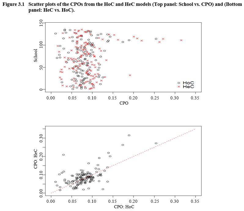
Description for Figure 3.1
Figure made of two scatter plots. The first compares the individual CPO values from the HeC and HoC models for each school. The school is on the y-axis, going from 0 to 150. CPOs are on the x-axis, going from 0.00 to 0.35. Most of the data points are concentrated between CPO values of 0.00 and 0.15 for both models.
The second graph compares the CPOs for HeC and HoC models. CPOs for HeC model are on the y-axis, ranging from 0.00 to 0.30. CPOs for HoC model are on the x-axis, ranging from 0.0 to 0.25. Generally CPO values for the HeC model are higher than those of HoC model.
Now, consider inference about
and
First, consider
Under the HoC
model, the posterior mean (PM) is 0.519, posterior standard deviation (PSD) is 0.068
and 95% credible interval (Cre) is (0.390, 0.639). Under the HeC model PM = 0.515,
PSD = 0.065 and 95% Cre is (0.383, 0.639). Second, consider
Under the HoC
model PM = 0.207, PSD = 0.011, and 95% Cre is (0.190,
0.224). Under the HeC model
PM = 0.208,
PSD = 0.011 and 95% Cre is (0.190, 0.225). Thus, it is good that
inference about
and
are very close for
the two competitors (HoC and HeC models).
In Table 3.2, we present posterior inference about the
finite population proportions for mathematics scores by areas. There are
differences between the posterior means under the HoC and HeC models. Most of
them are small but there are a few large differences. For NC, SR and CR, we
have 0.560 (0.543), 0.568 (0.584) and 0.465 (0.445) under the HoC (HeC) model,
respectively. The posterior standard deviations are also close but there are a
few moderately large differences (e.g., for NR we have 0.113 under the HoC
model and 0.077 under the HeC model). These differences are reflected in the
credible and highest posterior density (HPD) intervals.
Table 3.2
Comparison of posterior inference from the two-fold models with homogeneous correlation (HoC) and heterogeneous correlations (HeC) for the finite population proportions for US students below average in mathematics by area
Table summary
This table displays the results of Comparison of posterior inference from the two-fold models with homogeneous correlation (HoC) and heterogeneous correlations (HeC) for the finite population proportions for US students below average in mathematics by area. The information is grouped by Area (appearing as row headers), HoC Model and HeC Model (appearing as column headers).
| Area |
HoC Model |
HeC Model |
| PM |
PSD |
95% Cre |
95% HPD |
PM |
PSD |
95% Cre |
95% HPD |
| NR |
0.522 |
0.113 |
(0.299, 0.735) |
(0.310, 0.741) |
0.525 |
0.077 |
(0.363, 0.662) |
(0.361, 0.658) |
| NO |
0.365 |
0.075 |
(0.227, 0.524) |
(0.227, 0.520) |
0.359 |
0.072 |
(0.228, 0.511) |
(0.236, 0.516) |
| NC |
0.560 |
0.070 |
(0.420, 0.701) |
(0.408, 0.680) |
0.543 |
0.082 |
(0.370, 0.695) |
(0.396, 0.710) |
| SR |
0.568 |
0.080 |
(0.405, 0.725) |
(0.424, 0.731) |
0.584 |
0.062 |
(0.454, 0.699) |
(0.456, 0.699) |
| SO |
0.537 |
0.058 |
(0.423, 0.648) |
(0.417, 0.639) |
0.537 |
0.063 |
(0.409, 0.655) |
(0.408, 0.653) |
| SC |
0.646 |
0.064 |
(0.552, 0.766) |
(0.522, 0.766) |
0.654 |
0.059 |
(0.521, 0.763) |
(0.544, 0.774) |
| CR |
0.465 |
0.137 |
(0.195, 0.719) |
(0.185, 0.709) |
0.445 |
0.125 |
(0.212, 0.716) |
(0.199, 0.700) |
| CO |
0.437 |
0.085 |
(0.279, 0.603) |
(0.276, 0.596) |
0.439 |
0.091 |
(0.257, 0.620) |
(0.265, 0.620) |
| CC |
0.549 |
0.064 |
(0.415, 0.671) |
(0.423, 0.672) |
0.550 |
0.066 |
(0.414, 0.681) |
(0.422, 0.685) |
| WR |
0.461 |
0.086 |
(0.297, 0.629) |
(0.295, 0.626) |
0.460 |
0.085 |
(0.289, 0.626) |
(0.276, 0.611) |
| WO |
0.516 |
0.066 |
(0.384, 0.643) |
(0.387, 0.644) |
0.516 |
0.058 |
(0.401, 0.626) |
(0.409, 0.633) |
| WC |
0.670 |
0.042 |
(0.581, 0.748) |
(0.586, 0.749) |
0.662 |
0.047 |
(0.569, 0.748) |
(0.568, 0.746) |
Table 3.3 shows summaries of the PM, PSD and 95% HPD
for intracluster correlations under the HeC model. We can see that the
intracluster correlations vary over the areas. The largest estimate is 0.337
for NC and the smallest one is 0.073 for SR. Both areas have a few large
difference between the posterior means under the HoC and HeC models. The 95%
HPD interval for the common correlation in the HoC model is (0.160, 0.260) and
this interval is contained by all the intervals except for NR, NC, SR and WC.
Thus, it is reasonable to study the HeC model.
Table 3.3
Posterior summaries for the intracluster correlations of the two-fold models with heterogeneous correlations for US students below average in mathematics by area
Table summary
This table displays the results of Posterior summaries for the intracluster correlations of the two-fold models with heterogeneous correlations for US students below average in mathematics by area. The information is grouped by Area (appearing as row headers), PM , PSD , 95% Cre and 95% HPD (appearing as column headers).
| Area |
PM |
PSD |
95% Cre |
95% HPD |
| NR |
0.076 |
0.084 |
(0.002, 0.301) |
(0.001, 0.251) |
| NO |
0.184 |
0.087 |
(0.053, 0.380) |
(0.042, 0.358) |
| NC |
0.337 |
0.087 |
(0.190, 0.520) |
(0.184, 0.513) |
| SR |
0.073 |
0.067 |
(0.003, 0.252) |
(0.001, 0.216) |
| SO |
0.237 |
0.075 |
(0.113, 0.393) |
(0.110, 0.387) |
| SC |
0.176 |
0.079 |
(0.055, 0.356) |
(0.048, 0.329) |
| CR |
0.149 |
0.147 |
(0.003, 0.523) |
(0.001, 0.445) |
| CO |
0.233 |
0.103 |
(0.079, 0.486) |
(0.050, 0.434) |
| CC |
0.235 |
0.077 |
(0.105, 0.388) |
(0.099, 0.381) |
| WR |
0.181 |
0.099 |
(0.033, 0.413) |
(0.021, 0.378) |
| WO |
0.181 |
0.075 |
(0.059, 0.362) |
(0.048, 0.327) |
| WC |
0.301 |
0.063 |
(0.191, 0.437) |
(0.188, 0.434) |
In Figure 3.2, we compare
the posterior densities of the intracluster correlations (twelve correlations)
from the HeC model and the HoC model (one correlation). The distributions under
the HeC model are more variable and are mostly to the left or right of those
under the HoC model with not much overlap for some areas (e.g., NR, NC and SR).
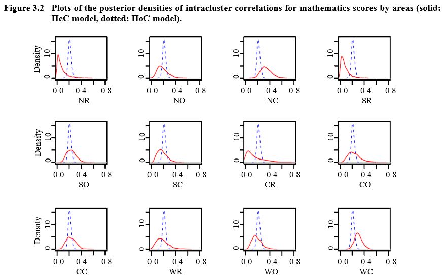
Description for Figure 3.2
Figure made of twelve graphs presenting the posterior densities of intracluster correlations for mathematics scores by areas (NR, NO, NC, SR, SO, SC, CR, CO, CC, WR, WO and WC) for HeC and HoC models. For each graph, density is on the y-axis, ranging from 0 to 15 and correlations are on the x-axis, ranging from 0.0 to 0.8. The distributions under the HeC model are more variable and are mostly to the left or right of those under the HoC model. Areas NR, NC and SR show a weak overlap between the two distributions. Areas NO, SC, CR, WR, WO and WC show an overlap a little bit bigger. Finally, densities for areas SO, CO and CC overlap more, but not completely.
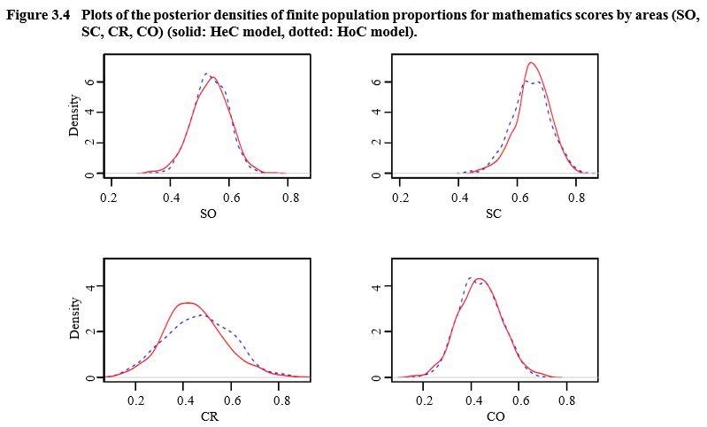
In Figures 3.3, 3.4 and 3.5, we compare the posterior
density plots of the finite population proportions for the mathematics score
and all areas for the two models. There are noticeable differences between the
HoC and HeC models (e.g., areas NR, NC, SR, CR and WC).
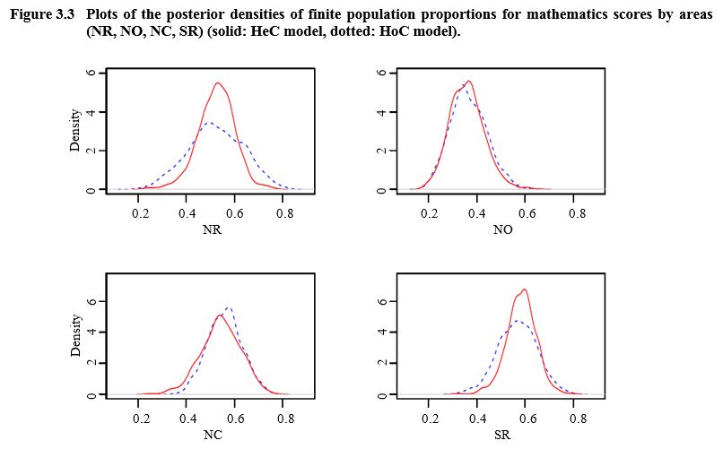
Description for Figure 3.3
Figure made of four graphs presenting the posterior densities of finite population proportions for mathematics scores by areas (NR, NO, NC and SR) for HeC and HoC models. For each graph, density is on the y-axis, ranging from 0 to 6 and proportions are on the x-axis, ranging from 0.0 to 0.8. There are noticeable differences between the HoC and HeC models for areas NR, NC and SR. The distributions are closer for area NO.
Description for Figure 3.4
Figure made of four graphs presenting the posterior densities of finite population proportions for mathematics scores by areas (SO, SC, CR and CO) for HeC and HoC models. For each graph, density is on the y-axis, ranging from 0 to 6 and proportions are on the x-axis, ranging from 0.0 to 0.8. There are noticeable differences between the HoC and HeC models for area CR. The distributions are closer for areas SO, SC and CO.
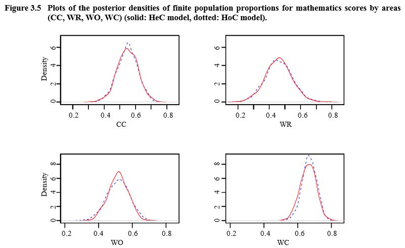
Description for Figure 3.5
Figure made of four graphs presenting the posterior densities of finite population proportions for mathematics scores by areas (CC, WR, WO and WC) for HeC and HoC models. For each graph, density is on the y-axis, ranging from 0 to 6 for CC and WR and from 0 to 8 for WO and WC and proportions are on the x-axis, ranging from 0.0 to 0.8. There are noticeable differences between the HoC and HeC models for area WC. The distributions are closer for areas CC, WR and WO.
3.2 Simulation study
In order to further
assess the performance of the HeC model and to compare it to the HoC model, we
perform a simulation study. Here we use two factors, each at three levels, to
get nine design points.
We have set 100 as the
number of clusters (schools) in each area and 15 as the number of individuals
(students) within each cluster. In other words, we take
where
Let
denote a vector
of posterior means and
denote the
vector of posterior standard deviations corresponding to the
or the
Specifically,
for the
we use
and
and for the
we use
and
When we
simulate data from the HeC model, the levels of the
are
and the levels
of the
are
For the twelve
areas
takes values 0.09,
0.19, 0.32, 0.08, 0.22, 0.18, 0.15, 0.22, 0.23, 0.17, 0.18, 0.30;
0.08, 0.09,
0.08, 0.06, 0.07, 0.08, 0.13, 0.09, 0.07, 0.09, 0.07, 0.06;
0.53, 0.37,
0.54, 0.58, 0.54, 0.65, 0.46, 0.44, 0.55, 0.46, 0.52, 0.66; and
0.08, 0.08,
0.08, 0.06, 0.06, 0.06, 0.12, 0.09, 0.07, 0.08, 0.06, 0.05.
We also take a simple
random sample of five clusters among the 100 population clusters, and a simple
random sample of ten individuals from each sampled cluster (i.e.,
and
These numbers
are much smaller than those of data used in Section 3.1, which makes inference
a little more challenging (Nandram 2015). Note that the dataset has about 7% of
the sampled clusters where all students were either below or above average. We
call this quantity the percent of sparseness. The setting of this simulation
study also leads to even sparser data. For nine design points, all the average
percents of sparseness are greater than 7% and most are around 10%. Figure 3.6
shows the histograms of sparseness percents for each design point.
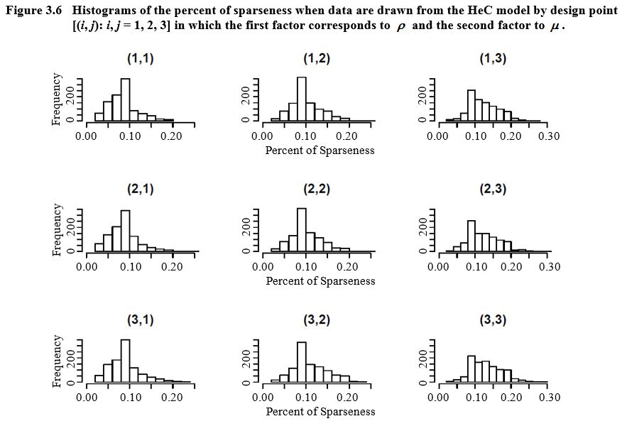
Description for Figure 3.6
Figure made of nine graphs presenting the histograms of the percent of sparseness when data are drawn from the HeC model by design point in which the first factor corresponds to and the second factor to For each graph, the frequency is on the y-axis ranging from 0 to 200 and the percent of sparseness is on the x-axis ranging from 0.00 to 0.30 when and from 0.00 to 0.20 otherwise. For the three graphs where the percent of sparseness peaks at about 10%, with a higher frequency below than above 10%. For the three graphs where the percent of sparseness peaks at about 10%, with a higher frequency above than below 10%. For the three graphs where the percent of sparseness peaks at about 10%, with a very low frequency for percent lower than 10%.
We consider two
scenarios. In the first scenario, we generate data from the HeC model and fit
both models, and in the second scenario, we generate data from the HoC model
and fit both models. When data are simulated from the HeC model, we have nine
design points
the first
factor corresponds to the
When we
simulate data from the HoC model, we have three design points
for the three
levels for the
is kept fixed
at its posterior mean.
In the first scenario, at
each design point we simulate binary data from the HeC model,
So we have the true values of
for
We take 1,000 samples at each of the nine
design points. For each sample we perform the blocked griddy Gibbs sampler in
the same manner as for the data.
Like Nandram (2015), we
calculate
and
to study the
frequentist properties of our procedure
We also obtain
the 95% credible interval and HPD interval for each of the 1,000 simulated
runs, and we study the width
and the credible
incidence
If the 95%
credible (or HPD) interval of
run contains
the true value
is equal to
one, otherwise it is equal to zero. Thus, the estimated probability content of
the 95% credible interval for the
area is
Table 3.4 shows
comparison of the HoC and HeC models. Under the HeC model the coverages are
much higher than those under the HoC model. Note that the coverages of HPD
intervals for the HeC model are much closer to the nominal value of 95% and
they are conservative. However, the 95% credible and HPD intervals are wider
than those from the HoC model. These effects are much larger as
becomes
larger. All measures AB, RAB and RPMSE under the HeC model are smaller than
those under the HoC model. Thus, based on these measures, the HeC model is
preferred over the HoC model.
Table 3.4
Simulation under the HeC model: Comparison of the HeC and HoC models using mean coverage and widths of 95% credible intervals and absolute bias, relative absolute bias and root posterior mean squared error for finite poulation proportions by design point
Table summary
This table displays the results of Simulation under the HeC model: Comparison of the HeC and HoC models using mean coverage and widths of 95% credible intervals and absolute bias. The information is grouped by Design Point (appearing as row headers), Model , C-Cre , W-Cre , C-HPD , W-HPD, AB , AB and RPMSE (appearing as column headers).
| Design Point |
Model |
C-Cre |
W-Cre |
C-HPD |
W-HPD |
AB |
RAB |
RPMSE |
| (1,1) |
HeC |
0.989 |
0.620 |
0.961 |
0.603 |
0.112 |
0.227 |
0.206 |
| HoC |
0.930 |
0.555 |
0.893 |
0.541 |
0.130 |
0.266 |
0.207 |
| (1,2) |
HeC |
0.984 |
0.622 |
0.960 |
0.603 |
0.112 |
0.227 |
0.206 |
| HoC |
0.926 |
0.558 |
0.889 |
0.545 |
0.132 |
0.249 |
0.209 |
| (1,3) |
HeC |
0.980 |
0.623 |
0.955 |
0.608 |
0 .120 |
0.211 |
0.210 |
| HoC |
0.923 |
0.558 |
0.892 |
0.546 |
0.134 |
0.236 |
0.212 |
| (2,1) |
HeC |
0.982 |
0.621 |
0.953 |
0.603 |
0.119 |
0.242 |
0.212 |
| HoC |
0.922 |
0.564 |
0.879 |
0.549 |
0.137 |
0.281 |
0.215 |
| (2,2) |
HeC |
0.980 |
0.625 |
0.952 |
0.609 |
0.122 |
0.228 |
0.214 |
| HoC |
0.918 |
0.566 |
0.879 |
0.552 |
0.139 |
0.264 |
0.217 |
| (2,3) |
HeC |
0.981 |
0.628 |
0.956 |
0.611 |
0.121 |
0.211 |
0.214 |
| HoC |
0.930 |
0.570 |
0.895 |
0.556 |
0.135 |
0.239 |
0.214 |
| (3,1) |
HeC |
0.982 |
0.627 |
0.949 |
0.608 |
0.121 |
0.245 |
0.215 |
| HoC |
0.934 |
0.583 |
0.892 |
0.566 |
0.136 |
0.278 |
0.218 |
| (3,2) |
HeC |
0.980 |
0.628 |
0.947 |
0.610 |
0.123 |
0.242 |
0.217 |
| HoC |
0.928 |
0.583 |
0.885 |
0.566 |
0.138 |
0.274 |
0.220 |
| (3,3) |
HeC |
0.976 |
0.632 |
0.951 |
0.614 |
0.124 |
0.218 |
0.218 |
| HoC |
0.928 |
0.581 |
0.889 |
0.565 |
0.139 |
0.246 |
0.220 |
In Table 3.5 we compare summaries of DIC, BPP and LPML.
All the DICs under the HeC model are smaller than the corresponding ones under
the HoC model and all the LPMLs under the HeC model are larger than those under
the HoC model. Under the HoC model, all the BPPs vary in (0.06, 0.09)
but under the HeC model they vary in (0.2, 0.4). Again, these measures show that the HeC model is
superior to the HoC model.
In a similar manner, for the second scenario we generate
binary data from
In Table 3.6 we present comparison of the HoC and HeC models. Here AB, RAB
and RPMSE are only slightly smaller under the HoC model. The coverages of the
credible and HPD intervals under the HeC model are closer to the nominal value
of 95%, while those under the HoC model are smaller. Table 3.7 shows summaries
of DIC, BPP and LPML. All the DICs under the HeC model are smaller than those
under the HeC model, while the BPPs and LPMLs are similar for the two models,
with those under the HoC model being slightly better.
Table 3.5
Simulation under the HeC model: Comparison of the HeC and HoC models using the deviance information criterion (DIC), the Bayesian predictive p-value (BPP) and the log pseudo marginal likelihood (LPML) by design point
Table summary
This table displays the results of Simulation under the HeC model: Comparison of the HeC and HoC models using the deviance information criterion (DIC). The information is grouped by Design Point (appearing as row headers), HoC Model and HeC Model (appearing as column headers).
| Design Point |
HoC Model |
HeC Model |
| DIC |
BPP |
LPML |
DIC |
BPP |
LPML |
| (1,1) |
419.275 |
0.090 |
-285.452 |
402.044 |
0.429 |
-267.990 |
| (1,2) |
418.351 |
0.091 |
-286.250 |
400.647 |
0.439 |
-266.377 |
| (1,3) |
416.784 |
0.088 |
-286.290 |
400.414 |
0.446 |
-267.203 |
| (2,1) |
436.980 |
0.067 |
-307.028 |
416.264 |
0.300 |
-292.756 |
| (2,2) |
437.306 |
0.062 |
-308.816 |
414.955 |
0.318 |
-292.404 |
| (2,3) |
430.531 |
0.080 |
-302.258 |
410.436 |
0.351 |
-285.206 |
| (3,1) |
441.204 |
0.090 |
-316.126 |
424.010 |
0.227 |
-308.825 |
| (3,2) |
442.165 |
0.083 |
-318.223 |
424.363 |
0.235 |
-309.815 |
| (3,3) |
438.305 |
0.071 |
-315.159 |
418.827 |
0.260 |
-306.619 |
Table 3.6
Simulation under the HoC model: Comparison of the HeC and HoC models using mean coverage and widths of 95% credible intervals and absolute bias, relative absolute bias and root posterior mean squared error for finite poulation proportions by design point
Table summary
This table displays the results of Simulation under the HoC model: Comparison of the HeC and HoC models using mean coverage and widths of 95% credible intervals and absolute bias. The information is grouped by Design Point (appearing as row headers), Model , C-Cre , W-Cre , C-HPD , W-HPD, AB , RAB and RPMSE (appearing as column headers).
| Design Point |
Model |
C-Cre |
W-Cre |
C-HPD |
W-HPD |
AB |
RAB |
RPMSE |
| 1 |
HeC |
0.985 |
0.627 |
0.969 |
0.608 |
0.117 |
0.242 |
0.212 |
| HoC |
0.944 |
0.575 |
0.919 |
0.559 |
0.107 |
0.240 |
0.210 |
| 2 |
HeC |
0.988 |
0.634 |
0.952 |
0.616 |
0.122 |
0.234 |
0.216 |
| HoC |
0.938 |
0.585 |
0.917 |
0.568 |
0.115 |
0.214 |
0.211 |
| 3 |
HeC |
0.977 |
0.628 |
0.940 |
0.611 |
0.126 |
0.222 |
0.218 |
| HoC |
0.933 |
0.572 |
0.908 |
0.556 |
0.113 |
0.202 |
0.208 |
Table 3.7
Simulation under the HoC model: Comparison of the HeC and HoC models using the deviance information criterion (DIC), the Bayesian predictive p-value (BPP) and the log pseudo marginal likelihood (LPML) by design point
Table summary
This table displays the results of Simulation under the HoC model: Comparison of the HeC and HoC models using the deviance information criterion (DIC). The information is grouped by Design Point (appearing as row headers), HoC Model and HeC Model (appearing as column headers).
| Design Point |
HoC Model |
HeC Model |
| DIC |
BPP |
LPML |
DIC |
BPP |
LPML |
| 1 |
428.647 |
0.308 |
-300.526 |
416.626 |
0.302 |
-303.001 |
| 2 |
430.113 |
0.371 |
-295.191 |
417.557 |
0.317 |
-296.531 |
| 3 |
429.598 |
0.379 |
-295.613 |
414.877 |
0.335 |
-297.250 |
Thus, when data actually
come from the HeC model, there are some important differences among the two
models, with the HeC model being preferred. However, when data actually come
from the HoC model, there are minor differences between the two models. Of
course, the HeC model (unequal correlations) has more parameters than the HoC
model (one correlation).
