
4.4 Measures of central tendency
4.4.2 Calculating the median
Text begins
The median is the value in the middle of a data set, meaning that 50% of data points have a value smaller or equal to the median and 50% of data points have a value higher or equal to the median. For a small data set, you first count the number of data points (n) and arrange the data points in increasing order. If the number of data points is uneven, you add 1 to the number of points and divide the results by 2 to get the rank of the data point whose value is the median. The rank is the position of the data point after the data set has been arranged in increasing order: the smallest value is rank 1, the second-smallest value is rank 2, etc.
Example 1 – Median time in 200 metres of a top running athlete
Imagine that a top running athlete in a typical 200-metre training session runs in the following times: 26.1 seconds, 25.6 seconds, 25.7 seconds, 25.2 seconds, 25.0 seconds, 27.8 seconds and 24.1 seconds. How would you calculate his median time?
Let’s start with arranging the values in increasing order:
| Rank | Times (in seconds) |
|---|---|
| 1 | 24.1 |
| 2 | 25.0 |
| 3 | 25.2 |
| 4 | 25.6 |
| 5 | 25.7 |
| 6 | 26.1 |
| 7 | 27.8 |
There are n = 7 data points, which is an uneven number. The median will be the value of the data points of rank
(n + 1) ÷ 2 = (7 + 1) ÷ 2 = 4.
The median time is 25.6 seconds.
If the number of data points is even, the median will be the average of the data point of rank n ÷ 2 and the data point of rank (n ÷ 2) + 1.
Example 2 – Median time in 200 metres of a top running athlete (Part 2)
Now suppose that the athlete runs his eighth 200-metre run with a time of 24.7 seconds. What is his median time now?
| Rank | Times (in seconds) |
|---|---|
| 1 | 24.1 |
| 2 | 24.7 |
| 3 | 25.0 |
| 4 | 25.2 |
| 5 | 25.6 |
| 6 | 25.7 |
| 7 | 26.1 |
| 8 | 27.8 |
There are now n = 8 data points, an even number. The median is the mean between the data point of rank
n ÷ 2 = 8 ÷ 2 = 4
and the data point of rank
(n ÷ 2) + 1 = (8 ÷ 2) +1 = 5
Therefore, the median time is (25.2 + 25.6) ÷ 2 = 25.4 seconds.
For larger data sets, the cumulative relative frequency distribution can be helpful to identify the median. The median is the smallest value for which the cumulative relative frequency is at least 50%. However, when possible it’s best to use the basic statistical function available in a spreadsheet or statistical software application because the results will then be more reliable.
Example 3 – Median size of households of the students in the class
Imagine you ask the 30 students of your class how many people there are in their households. You summarize the data you collected in a frequency table, in which you include the relative frequencies and the cumulative relative frequencies.
| Household size | Frequency (number of students) | Relative frequency (%) | Cumulative frequency (number of students) | Cumulative relative frequency (%) |
|---|---|---|---|---|
| 2 | 3 | 10.0 | 3 | 10.0 |
| 3 | 4 | 13.3 | 7 | 23.3 |
| 4 | 10 | 33.3 | 17 | 56.7 |
| 5 | 4 | 13.3 | 21 | 70.0 |
| 6 | 2 | 6.7 | 23 | 76.7 |
| 7 | 3 | 10.0 | 26 | 86.7 |
| 8 | 1 | 3.3 | 27 | 90.0 |
| 9 | 2 | 6.7 | 29 | 96.7 |
| 10 | 1 | 3.3 | 30 | 100.0 |
You can see that 10% of students (3 students) live in a household of size 2, 23% of students (7 students) live in a household of size 3 or less and 57% of students (17 students) live in a household of size 4 or less. The median will be equal to 4 because it’s the smallest value for which the cumulative relative frequency is higher than 50%. This is even more obvious if you visualize the cumulative relative frequency on a bar chart like on chart 4.4.2.1. The dotted line indicates the cumulative relative frequency of 50%.
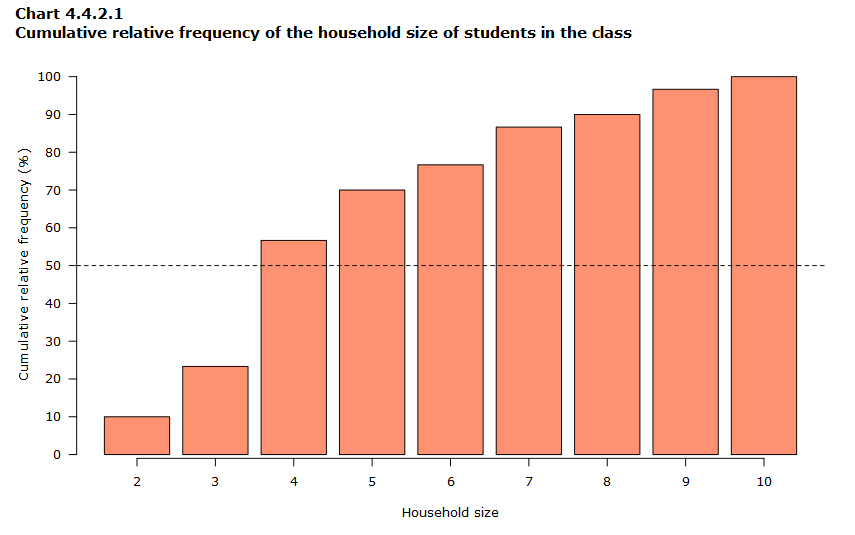
Data table for Chart 4.4.2.1
| Household size | Cumulative relative frequency (%) |
|---|---|
| 2 | 10.0 |
| 3 | 23.3 |
| 4 | 56.7 |
| 5 | 70.0 |
| 6 | 76.7 |
| 7 | 86.7 |
| 8 | 90.0 |
| 9 | 96.7 |
| 10 | 100.0 |
The mean is the total number of people in the households of the students:
2 × 3 + 3 × 4 + 4 × 10 + 5 × 4 + 6 × 2 + 7 × 3 + 8 × 1 + 9 × 2 + 10 × 1 = 147
divided by the number of students, which is 30. The result is 147 ÷ 30 = 4.9 people per household.
In this example, the median (4) is lower than the mean (4.9).
The advantage of using the median instead of the mean is that the median is more robust, which means that an extreme value added to one extremity of the distribution don’t have an impact on the median as big as the impact on the mean. Therefore, it is important to check if the data set includes extreme values before choosing a measure of central tendency. This will be illustrated by the next example.
Example 4 – Median size of households of the students in the class (Part 2)
A new student recently joined your class. You decide to ask him what the size of his household is in order to update your results. He replies to you that he lives in a large multi-generational house that includes 18 people!
Once updated, the mean is (147 + 18) ÷ 31 = 5.3 people per household. Just adding one new student increased the mean by 0.4 (5.3 – 4.9). The median is the same after the update. There are now 7 ÷ 31 = 22.6% of students in a household of size 3 or less, and 17 ÷ 31 = 54.8% of students that live in a household of size 4 or less. The value 4 is still the smallest value with a cumulative relative frequency of at least 50%.
- Date modified: