
4 Data exploration
4.3 Frequency distribution
Text begins
The frequency (f) of a particular value is the number of times the value occurs in the data. The distribution of a variable is the pattern of frequencies, meaning the set of all possible values and the frequencies associated with these values. Frequency distributions are portrayed as frequency tables or charts.
Frequency distributions can show either the actual number of observations falling in each range or the percentage of observations. In the latter instance, the distribution is called a relative frequency distribution.
Frequency distribution tables can be used for both categorical and numeric variables. Continuous variables should only be used with class intervals, which will be explained shortly.
Let’s look at some examples of frequency distribution and relative frequency distribution for discrete variables.
Example 1 – Constructing a frequency distribution table
A survey was taken on Maple Avenue. In each of 20 homes, people were asked how many cars were registered to their households. The results were recorded as follows:
1, 2, 1, 0, 3, 4, 0, 1, 1, 1, 2, 2, 3, 2, 3, 2, 1, 4, 0, 0
Use the following steps to present this data in a frequency distribution table.
- Divide the results (x) into intervals, and then count the number of results in each interval. In this case, the intervals would be the number of households with no car (0), one car (1), two cars (2) and so forth.
- Make a table with separate columns for the interval numbers (the number of cars per household), the tallied results, and the frequency of results in each interval. Label these columns Number of cars, Tally and Frequency.
- Read the list of data from left to right and place a tally mark in the appropriate row. For example, the first result is a 1, so place a tally mark in the row beside where 1 appears in the interval column (Number of cars). The next result is a 2, so place a tally mark in the row beside the 2, and so on. When you reach your fifth tally mark, draw a tally line through the preceding four marks to make your final frequency calculations easier to read.
- Add up the number of tally marks in each row and record them in the final column entitled Frequency.
Your frequency distribution table for this exercise should look like this:
| Number of cars (x) | Frequency (f) |
|---|---|
| 0 | 4 |
| 1 | 6 |
| 2 | 5 |
| 3 | 3 |
| 4 | 2 |
| 0 true zero or a value rounded to zero | |
By looking at this frequency distribution table quickly, we can see that out of 20 households surveyed, 4 households had no cars, 6 households had 1 car, etc.
Example 2 – Constructing a cumulative frequency distribution table
A cumulative frequency distribution table is a more detailed table. It looks almost the same as a frequency distribution table but it has added columns that give the cumulative frequency and the cumulative percentage of the results, as well.
At a recent chess tournament, all 10 of the participants had to fill out a form that gave their names, address and age. The ages of the participants were recorded as follows:
36, 48, 54, 92, 57, 63, 66, 76, 66, 80
Use the following steps to present these data in a cumulative frequency distribution table.
- Divide the results into intervals, and then count the number of results in each interval. In this case, intervals of 10 are appropriate. Since 36 is the lowest age and 92 is the highest age, start the intervals at 35 to 44 and end the intervals with 85 to 94.
- Create a table similar to the frequency distribution table but with three extra columns.
- In the first column or the Lower value column, list the lower value of the result intervals. For example, in the first row, you would put the number 35.
- The next column is the Upper value column. Place the upper value of the result intervals. For example, you would put the number 44 in the first row.
- The third column is the Frequency column. Record the number of times a result appears between the lower and upper values. In the first row, place the number 1.
- The fourth column is the Cumulative frequency column. Here we add the cumulative frequency of the previous row to the frequency of the current row. Since this is the first row, the cumulative frequency is the same as the frequency. However, in the second row, the frequency for the 35–44 interval (i.e., 1) is added to the frequency for the 45–54 interval (i.e. 2). Thus, the cumulative frequency is 3, meaning we have 3 participants in the 34 to 54 age group.
1 + 2 = 3
- The next column is the Percentage column. In this column, list the percentage of the frequency. To do this, divide the frequency by the total number of results and multiply by 100. In this case, the frequency of the first row is 1 and the total number of results is 10. The percentage would then be 10.0.
10.0. (1 ÷ 10) X 100 = 10.0
- The final column is Cumulative percentage. In this column, divide the cumulative frequency by the total number of results and then to make a percentage, multiply by 100. Note that the last number in this column should always equal 100.0. In this example, the cumulative frequency is 1 and the total number of results is 10, therefore the cumulative percentage of the first row is 10.0.
10.0. (1 ÷ 10) X 100 = 10.0
The cumulative frequency distribution table should look like this:
Table 4.3.2
Ages of participants at a chess tournament
Table summary
This table displays the results of Ages of participants at a chess tournament. The information is grouped by Lower Value (appearing as row headers), Upper Value, Frequency (f), Cumulative frequency, Percentage and Cumulative percentage (appearing as column headers).Lower Value Upper Value Frequency (f) Cumulative frequency Percentage Cumulative percentage 35 44 1 1 10.0 10.0 45 54 2 3 20.0 30.0 55 64 2 5 20.0 50.0 65 74 2 7 20.0 70.0 75 84 2 9 20.0 90.0 85 94 1 10 10.0 100.0
Class intervals
If a variable takes a large number of values, then it is easier to present and handle the data by grouping the values into class intervals. Continuous variables are more likely to be presented in class intervals, while discrete variables can be grouped into class intervals or not.
To illustrate, suppose we set out age ranges for a study of young people, while allowing for the possibility that some older people may also fall into the scope of our study.
The frequency of a class interval is the number of observations that occur in a particular predefined interval. So, for example, if 20 people aged 5 to 9 appear in our study's data, the frequency for the 5–9 interval is 20.
The endpoints of a class interval are the lowest and highest values that a variable can take. So, the intervals in our study are 0 to 4 years, 5 to 9 years, 10 to 14 years, 15 to 19 years, 20 to 24 years, and 25 years and over. The endpoints of the first interval are 0 and 4 if the variable is discrete, and 0 and 4.999 if the variable is continuous. The endpoints of the other class intervals would be determined in the same way.
Class interval width is the difference between the lower endpoint of an interval and the lower endpoint of the next interval. Thus, if our study's continuous intervals are 0 to 4, 5 to 9, etc., the width of the first five intervals is 5, and the last interval is open, since no higher endpoint is assigned to it. The intervals could also be written as 0 to less than 5, 5 to less than 10, 10 to less than 15, 15 to less than 20, 20 to less than 25, and 25 and over.
Rules for data sets that contain a large number of observations
In summary, follow these basic rules when constructing a frequency distribution table for a data set that contains a large number of observations:
- find the lowest and highest values of the variables
- decide on the width of the class intervals
- include all possible values of the variable.
In deciding on the width of the class intervals, you will have to find a compromise between having intervals short enough so that not all of the observations fall in the same interval, but long enough so that you do not end up with only one observation per interval.
It is also important to make sure that the class intervals are mutually exclusive and collectively exhaustive.
Example 3 – Constructing a frequency distribution table for large numbers of observations
Thirty AA batteries were tested to determine how long they would last. The results, to the nearest minute, were recorded as follows:
423, 369, 387, 411, 393, 394, 371, 377, 389, 409, 392, 408, 431, 401, 363, 391, 405, 382, 400, 381, 399, 415, 428, 422, 396, 372, 410, 419, 386, 390
Use the steps in Example 1 and the above rules to help you construct a frequency distribution table.
Answer
The lowest value is 363 and the highest is 431.
Using the given data and a class interval of 10, the interval for the first class is 360 to 369 and includes 363 (the lowest value). Remember, there should always be enough class intervals so that the highest value is included.
The completed frequency distribution table should look like this:
| Battery life, minutes (x) | Frequency (f) |
|---|---|
| 360–369 | 2 |
| 370–379 | 3 |
| 380–389 | 5 |
| 390–399 | 7 |
| 400–409 | 5 |
| 410–419 | 4 |
| 420–429 | 3 |
| 430–439 | 1 |
| Total | 30 |
Example 4 – Constructing relative frequency and percentage frequency tables
An analyst studying the data from example 3 might want to know not only how long batteries last, but also what proportion of the batteries falls into each class interval of battery life.
This relative frequency of a particular observation or class interval is found by dividing the frequency (f) by the number of observations (n): that is, (f ÷ n). Thus:
Relative frequency = frequency ÷ number of observations
The percentage frequency is found by multiplying each relative frequency value by 100. Thus:
Percentage frequency = relative frequency X 100 = f ÷ n X 100
Use the data from Example 3 to make a table giving the relative frequency and percentage frequency of each interval of battery life.
Here is what that table looks like:
| Battery life, minutes (x) | Frequency (f) | Relative frequency | Percent frequency |
|---|---|---|---|
| 360–369 | 2 | 0.07 | 7 |
| 370–379 | 3 | 0.1 | 10 |
| 380–389 | 5 | 0.17 | 17 |
| 390–399 | 7 | 0.23 | 23 |
| 400–409 | 5 | 0.17 | 17 |
| 410–419 | 4 | 0.13 | 13 |
| 420–429 | 3 | 0.1 | 10 |
| 430–439 | 1 | 0.03 | 3 |
| Total | 30 | 1 | 100 |
An analyst of these data could now say that:
- 7% of AA batteries have a life of from 360 minutes up to but less than 370 minutes, and that
- the probability of any randomly selected AA battery having a life in this range is approximately 0.07.
Example 5 – Visualization of the cumulative relative frequency distribution
As previously shown for example 2, cumulative frequency is used to determine the number of observations that lie below a particular value in a data set. The cumulative frequency is calculated by adding each frequency from a frequency distribution table to the sum of its predecessors. The last value will always be equal to the total for all observations, since all frequencies will already have been added to the previous total. Let’s look at another example of how to calculate the cumulative frequency.
The daily number of rock climbers in Lake Louise, Alberta was recorded over a 30-day period. The results are as follows:
31, 49, 19, 62, 24, 45, 23, 51, 55, 60, 40, 35 54, 26, 57, 37, 43, 65, 18, 41, 50, 56, 4, 54, 39, 52, 35, 51, 63, 42.
The number of rock climbers ranges from 4 to 65. In order to create a frequency table, the data are best grouped in class intervals of 10. Each interval can be one row in the frequency table. The Frequency column lists the number of observations found within a class interval. For example, there are only two values in the interval from 10 to 20, then its frequency is 2 in the table accordingly.
Use the Frequency column to calculate cumulative frequency.
- First, add the number from the Frequency column to its predecessor. For example, in the first row, we have only one observation and no predecessors. The cumulative frequency is one.
1 + 0 = 1 - However, in the second row, there are two observations. Add these two to the previous cumulative frequency (one), and the result is three.
1 + 2 = 3 - Record the results in the Cumulative frequency column.
The other entries in the table can be calculated similarly. Results are presented in the table 4.3.5.
| Number of rock climbers | Frequency (f) | Cumulative frequency |
|---|---|---|
| <10 | 1 | 1 |
| 10 to <20 | 2 | 1 + 2 = 3 |
| 20 to <30 | 3 | 3 + 3 = 6 |
| 30 to <40 | 5 | 6 + 5 = 11 |
| 40 to <50 | 6 | 11 + 6 = 17 |
| 50 to <60 | 9 | 17 + 9 = 26 |
| >= 60 | 4 | 26 + 4 = 30 |
Cumulative relative frequency is another way of expressing frequency distribution. It is obtained by calculating the percentage of the cumulative frequency within each interval.
Cumulative percentage is calculated by dividing the cumulative frequency by the total number of observations (n), then multiplying it by 100 (the last value will always be equal to 100%). Thus,
cumulative relative frequency = (cumulative frequency ÷ n) x 100
The fourth column in the table 4.3.6 shows the calculation of the cumulative relative frequency of the daily number of rock climbers recorded in Lake Louise.
| Number of rock climbers | Frequency (f) | Cumulative frequency | Cumulative relative frequency (%) |
|---|---|---|---|
| <10 | 1 | 1 | 1 ÷ 30 x 100 = 3 |
| 10 to <20 | 2 | 1 + 2 = 3 | 3 ÷ 30 x 100 = 10 |
| 20 to <30 | 3 | 3 + 3 = 6 | 6 ÷ 30 x 100 = 20 |
| 30 to <40 | 5 | 6 + 5 = 11 | 11 ÷ 30 x 100 = 37 |
| 40 to <50 | 6 | 11 + 6 = 17 | 17 ÷ 30 x 100 = 57 |
| 50 to <60 | 9 | 17 + 9 = 26 | 26 ÷ 30 x 100 = 87 |
| >= 60 | 4 | 26 + 4 = 30 | 30 ÷ 30 x 100 = 100 |
The cumulative relative frequency distribution can be visualized with a bar chart or a line chart, like in chart 4.3.1 below. The value on the horizontal axis is the upper bound of the class interval.
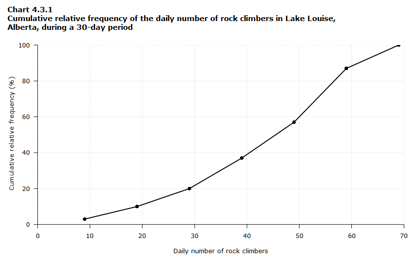
Data table for Chart 4.3.1
| Upper bound of the class interval of daily number of rock climbers | Cumulative relative frequency (%) |
|---|---|
| 9 | 3 |
| 19 | 10 |
| 29 | 20 |
| 39 | 37 |
| 49 | 57 |
| 59 | 87 |
| 69 | 100 |
Chart 4.3.1 shows that for the majority of days (57%) in the period, the number of rock climbers was lower or equal to 49.
Frequency distribution can be visualized using:
- a pie chart (nominal variable),
- a bar chart (nominal or ordinal variable),
- a line chart (ordinal or discrete variable),
- or a histogram (continuous variable).
These types of charts will be presented in the section 5 on data visualization. But first, we will look at other methods to summarize data using measures of central tendency and dispersion.
- Date modified: