2 Methodology

Stephen J. Kaputa and Katherine Jenny Thompson

Previous | Next

2.1  Decile estimation

We consider two approaches to decile estimation for continuous data: the sample decile (SD) method and interpolation. The SD method uses ordered sample weights to locate the estimate (Rao and Shao 1996). For this, the characteristics values are sorted in ascending order, and the sample weights are accumulated until they exceed the desired decile's percent of the total weight.

Interpolation methods group the continuous data in bins and interpolate over the bin containing the decile. To obtain the decile estimate $\left({\xi }^d\right),$ we use the Woodruff formula (Woodruff 1952) for interpolation provided below:

$${\xi }^d=F^{-1}\left(d\widehat{N}\right)\approx ll+\left(\frac{d\widehat{N}-cf}{f_i}\right)*(i)\left(2.1\right)$$

where

$F=$ cumulative frequency of the characteristic using sample weights,

$ll=$ lower limit of the bin containing the decile,

$\widehat{N}=$ estimated total number of elements in the population,

$cf=$ cumulative frequency in all intervals preceding the bin containing the sample decile,

$f_i=$ decile class frequency (estimated total number of elements in the population of the interval containing the sample decile),

$i=$ width of the bin containing the sample decile,

$d=$ desired decile (0.1, 0.2, 0.3, … , 0.9).

Notice that this formula does not require that each bin to be of equal length. However, it does require that the data within each bin be uniformly distributed. This later requirement poses the true challenge with a highly skewed population, especially in the upper tail.

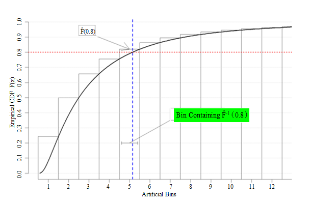
Figure 2.1 below illustrates how to use the Woodruff method to estimate the 80^th decile. The sample data have been grouped into twelve separate bins. The empirical CDF is produced from the complete set of weighted sample data (as one referee noted, the empirical CDF is extremely smooth for sample survey data; in practice, the curve would include discrete steps. The Woodruff method procedure would be the same, however). The decile estimate is located at the intersection of the empirical CDF curve and red asymptote at $\text{Y}=\mathrm{0.80.}$ The 80^th decile is ${\text{F}}^{-1}(0.80),$ contained in the 5^th bin; the interpolated estimate of the 80^th percentile would therefore be obtained by using (2.1) over the fifth bin.

Description for figure 2.1

Figure 2.1 Illustration of the Woodruff method

Determining the optimal bin size for both estimation and variance estimation can be difficult. As the bins narrow (approaching width 1), then the variance estimates become more unstable. Smoothing the estimates via the interpolation reduces the instability of variance, but increases the bias in the estimate. The bias component increases as the bin widths increase.

Economic data generally have a positive skewed distribution. Moreover, the subdomains' characteristic distributions will vary, and their respective moments change over time as the economy changes. Consequently, developing a standard set of fixed bins for interpolation that work consistently over time is nearly impossible. Instead, Thompson and Sigman (2000) developed a "data-dependent� binning procedure, where the width of each bin is determined separately by the estimation cell. Their recommended method linearly transforms each characteristic to a standard scale and then uses a standard set of bins for every characteristic. The authors use the following linear transformation

$$X_i^{\prime }=X_i\times \frac{1,000}{Q_{75}}$$

where $Q_{75}$ is the 75^th percentile (3^rd quartile) of the sample distribution, obtained using the SD method. The interpolated-median estimate of the $X^{\prime }$ is multiplied by $(Q_{75}/1,000)$ to obtain a value on the original scale. This procedure is equivalent to simply dividing the original sample in each estimation cell from 0 to $Q_{75}$ into $Z$ bins of equal width and placing the remainder of the sample into one bin, which, by design, is much larger than the others. With the highly positive skewed housing data, this transformation works well for estimating the median because it is far from the $Q_{75}$ scaling parameter. However, it does not permit estimation of either the 80^th or 90^th deciles. Thus, if we wanted to continue using an interpolation method, we needed to consider alternative transformations.

The simplest approach is to use the original data-dependent bin method with a higher scaling parameter, i.e., use any percentile value larger than 90%. We use the 95^th percentile as the scaling factor and hereafter refer to this method as the "P95 method�.

The P95 method does create uniform distributions within the majority of the bins but is still problematic at the upper end of the distribution for two reasons. First, the final bin contains only five percent of the sample distribution, and the values within this bin are generally very different. Second, the data-dependent binning procedure requires that each decile be "far from� the large final bin; if not, then the decile estimates exhibit the same instability as those obtained using the "SD method�. Unfortunately, the bin containing the 90^th percentile is often close to the final bin when using a scaling parameter of 95%.

To address the second issue, we considered another data-binning approach, denoted as the "P75 method�. For this, we create two sets of bins per estimation cell, each with different widths above and below the cell's $Q_{75}$ value. This requires two separate linear transformations per estimation cell, given by

$$\begin{array}{l}{X}_i^{\prime }=X_i\times \frac{1,000}{X_{75}}\text{ when }{X}_i<X_{75}\\ X_i^{″}=\left(X_i-X_{75}\right)\times \frac{1,000}{\left(X_{100}-X_{75}\right)}\\ \text{ when }{X}_i\ge X_p\text{ and }{X}_{100}=\text{maximum value in sample}\text{.}\end{array}$$

The $X_i^{\prime }$ is then placed into $Z$ equal length bins, and $X_i^{″}$ into $K$ equal length bins, where $Z\ne K.$ The interpolation is performed independently for each decile, with the appropriate inverse transformation being applied to each interpolated decile. This procedure ensures that median estimates exactly match those obtained with the current procedure.

Our third considered interpolation approach makes parametric assumptions about the characteristics. Often, economic data are approximately log-normally distributed (e.g., Steel and Fay 1995). The Normal Binning method (denoted "NB�) uses the properties of the normal distribution applied to the log-transformed data to obtain data-dependent bins. The binning technique ensures that areas of high probability have smaller bin widths to limit the amount of observations per bin and areas of low probability have larger bin width to increase the amount of observations per bin.

The NB method centers the log-transformed data around the weighted sample median, then scales the centered data by an estimate of the population standard deviation. We use the sample median because it is more outlier resistant than the sample mean. Of course, the mean and median are equivalent with normally distributed data. Given a standard normal distribution where $\mu =0$ and $\sigma =1,$ then

$$\begin{array}{l}IQR=Q_3-Q_1\\ IQR=\left(\text{0}\text{.67449*}\sigma \right)-\left(\text{-0}\text{.67449*}\sigma \right)=\sigma \left(\text{0}\text{.67449}+\text{0}\text{.67449}\right)=\sigma *\mathrm{1.34898.}\end{array}$$

We estimated the standard deviation (sigma) as the ratio $\sigma \approx IQR/1.34898,$ where the IQR is obtained from the empirical CDF in the estimation cell. To normalize the data, we applied the following transformation

$$Y_i=\text{Log}\left(X_i\right)$$

$$\left[{Y^{\prime }}_i=\frac{Y_i-Y_{\text{med}}}{{\sigma }_y}=\frac{Y_i-Y_{\text{med}}}{IQ{R}_y/1.34898}\right]$$

where

$Y_{\text{med}}=$ log-transformed sample median over domain $i,$

$IQ{R}_y=$ log-transformed sample interquartile range over domain $i.$

Again, the sample deciles and interquartile ranges are obtained via the SD method. If the data are log-normally distributed, $Y_i^{\prime }$ should have a standard normal distribution, so that roughly 68.3% of the data are within one standard deviation of the mean and 95.4% of the data are within two standard deviations of the mean. Using those properties, we split the transformed $Y_i^{\prime }$ into the five different zones and created the 45 bins shown in Table 2.1.

Table 2.1
Bins for the log-normal transformation (Normal method)
Table summary
This table displays Bins for the log-normal transformation. The information is grouped by zone (appearing as row headers), 1, 2, 3, 4, 5 (appearing as column headers).

Zone	1	2	3	4	5
Range	[Low, -2)	[-2, -1)	[-1, 1)	[1, 2)	[2, High]
Percent in Zone	2.3	13.6	68.2	13,6	2.3
Bins	1	6	31	6	1
Average Percent of Sample Units per Bin	2.3	2.3	2.2	2,3	2.3

There are four different bin widths with roughly the same average percentage of sampled units per bin. Woodruff's method is applied to the transformed data to obtain the deciles and we exponentiate these decile estimates to obtain values on the original scale. Unlike the linear rescaling methods presented above, there is an additional induced estimation bias caused by the power transformation. It may have been possible to make a bias adjustment for the transformation via a Taylor expansion, as suggested by a referee, but we did not consider this approach.

2.2  Variance estimation

The MHS replication method (aka "Fay's method�) is a "compromise� between the stratified jackknife and the BRR method (Fay 1989). Rao and Shao (1999) demonstrate that the MHS variance estimator is asymptotically consistent for both smooth statistics such as ratio estimators and for non-smooth statistics such as sample quantiles estimated using the SD method outlined in 2.1. Their paper does not extend this property to interpolated decile estimates, although it does follow that these variance estimates should be consistent as the bin width approaches width 1. Like BRR, MHS replication uses a Hadamard matrix to form replicates, but uses replicate weights of 1.5 and 0.5 instead of the values of 2 and 0 used in BRR. The MHS formula for standard error estimation of any estimate $\widehat{\theta }$ is

$$\widehat{S}(\widehat{\theta })=\sqrt{\frac{4}{R}*{\displaystyle \sum _{r=1}^R{({\widehat{\theta }}_r-{\widehat{\theta }}_0)}^2}}\left(2.2\right)$$

where ${\widehat{\theta }}_r$ is the $r^{\text{th}}$ replicate estimate $(r=1,2,\dots ,R)$ and ${\widehat{\theta }}_0$ is the full sample estimate. The sum of squared error term is adjusted by a factor of $4=1/{\left(1-0.5\right)}^2$ to prevent negative bias in the variance estimate (Judkins 1990).

Previous | Next