
Latest Developments in the Canadian Economic Accounts
Results from the 2015 Comprehensive Revision to the Canadian System of Macroeconomic Accounts

Archived Content
Information identified as archived is provided for reference, research or recordkeeping purposes. It is not subject to the Government of Canada Web Standards and has not been altered or updated since it was archived. Please "contact us" to request a format other than those available.

1. Background
Statistical revisions are carried out regularly in the Canadian System of Macroeconomic Accounts (CSMA), in order to incorporate the most current information from censuses, annual surveys, administrative statistics, public accounts and other sources. Generally, these revisions are limited to the months or quarters within a given reference year, or, on an annual basis, to two to three years to incorporate benchmark information.
Periodically, more comprehensive revisions are conducted. These provide an opportunity to improve estimation methods, incorporate improved data sources, introduce conceptual changes and adopt new international standards into the CSMA. These revisions generally cover a longer time period that is beyond the scope of annual revisions. Comprehensive revisions will be included in releases of the Canadian System of Macroeconomic Accounts starting in November 2015. The revisions are carried back to 1981 for some components, with the majority of revisions made from 2007 onwards.
Over the last number of years, the CSMA has been updated to reflect the latest international recommendations for macroeconomic accounting. These revisions are directly related to changes made to the international standards that are used by Statistics Canada and other national statistical organizations (such as the Bureau of Economic Analysis in the United States) to compile many Key macroeconomic indicators/datasets. This includes the System of National Accounts 2008 (SNA2008) used to compile the Canadian System of National Accounts, the Balance of Payments Manual Version 6 (BPM6) and the Foreign Direct Investment used to compile the Canadian International Accounts and the Government Finance Statistics Manual 2014 used to compile the Canadian Government Finance Statistics.
There are four main sources of revision with this release of the Canadian System of Macroeconomic Accounts: The integration of Government Finance Statistics, the improved treatment of defined benefit pension plans, the measurement of financial services purchased by households’, and updated measures of national wealth.
The largest source of the revision is a result of the incorporation of new and improved estimates of Government Finance Statistics. Over the last number of years Statistics Canada has modernized its government finance statistics program. This included adopting the concepts and accounting methods outlined in the International Monetary Fund’s (IMF) government accounting manual (the Government Finance Statistics Manual 2014) as well as incorporating improved and more detailed electronic data sources, particularly for provincial, territorial and local general governments. The new accounting concepts and methods and improved data sources have resulted in more accurate measures of government revenue, expenses, operating balances, assets and liabilities.
A second significant source of revision revolves around the treatment of defined benefit pension plans. In the previous version of the Canadian System of Macroeconomic Accounts the contributions to defined benefit pension plans were treated on a cash basis. This meant that the accumulated pension asset reflected the cash contributions plus the investment income of the plan – which may have understated or overstated the true contractual obligation of the defined benefit pension plans. The cash based treatment does not align with international macroeconomic accounting standards which recommend that pension benefits be recorded on an accrual basis. With the 2015 release of the Canadian System of Macroeconomic Accounts all payments to defined benefit pension plans are now treated on an accrual basis, meaning the pension accruals are recorded as income when the work is performed. This ensures that the compensation of employees aligns with the work performed and the pension asset built up in the household sector reflects the contractual obligations of employers with employees.
Another important revision involves the treatment of financial services purchased by households. New data sources indicate that the level of household purchases of explicit financial services was underreported in the previous version of the Canadian System of Macroeconomic Accounts. These new data show that the previous estimate of explicit financial services purchased by businesses was too high and the estimate of explicit financial services purchased by household was too low. The revision therefore reflects a reallocation from businesses to households which has the effect of increasing gross domestic product. In addition, previous estimates of investment dealer fees paid by households were too low. Improved data on mutual fund assets, incomes and administrative fees resulted in upward revisions.
The fourth revision relates to improvements to various aspects of the measurement of wealth on the National Balance Sheet Accounts:
- Natural resource wealth has been added to the quarterly National Balance Sheet Account. The addition of this asset improves the overall understanding of the capital used to produce goods and services. In addition to adding to Canada’s measure of wealth, this asset has also been apportioned between the government and non-financial corporations’ sector. The ‘sectoring’ of this asset ensures a more accurate measure of the net worth in both the corporate and government sectors.
- A second revision to wealth involves the incorporation of the latest benchmark estimates from the Survey of Financial Security and Property Assessment files to estimate the value of residential real estate. Previous estimates of the value of residential real estate were derived using the perpetual inventory method where the value of residential real estate is calculated by accumulating (and depreciating) residential investment flows and then using a land to structure ratio to derive the estimate of land. This methodology relies heavily on the new housing price index to calculate the market value of residential real estate. Analysis of the data against other sources indicated that the information from the Survey of Financial Security and the Property Assessment files provides a better measure of the market value of Canadian residential real estate.
- Finally, revised estimates of services lives for many of Canada’s non-residential assets and machinery and equipment were revised. In general these revisions resulted in an upward revision to the consumption fixed capital and a downward revision to the net capital stock of non-residential and machinery and equipment assets.
This paper provides users with a detailed explanation and reconciliation between previously published figures and the new revised figures.
2. Revisions to the level of gross domestic product
Although neither the asset or production boundary (key concepts in macroeconomic accounting determining what ultimately gets included in gross domestic product and national wealth) changed with this comprehensive revision, the average level of GDP was revised upward between 1981 and 2009 and downward between 2010 and 2014. Table 1 shows the change in the level of GDP for the period 1981 to 2014 broken down by revisions due to general government final consumption expenditure, household final consumption expenditure on services and other revisions.
| Time period | Revised average level of gross domestic product | Previously published average level of gross domestic product | Average revision to the level of gross domestic product | Average revision due to revisions to government final consumption expenditure | Average revision due to revisions to household final consumption expenditure on services | Average revision due to components other than revisions to government final consumption expenditure and household final consumption expenditure on services |
|---|---|---|---|---|---|---|
| millions of dollars | ||||||
| 1981 to 1989 | 502,412 | 500,842 | 1,570 | 1,380 | 404 | -215 |
| 1990 to 1999 | 817,403 | 815,015 | 2,389 | 930 | 1,328 | 131 |
| 2000 to 2009 | 1,371,689 | 1,365,922 | 5,766 | -73 | 4,795 | 1,045 |
| 2010 to 2014 | 1,824,019 | 1,826,517 | -2,498 | -9,848 | 7,649 | -298 |
| Average of all years | 1,045,080 | 1,042,633 | 2,447 | -831 | 3,033 | 245 |
| Source: Statistics Canada. | ||||||
The move by governments to new accrual-based public sector accounting standards and Statistics Canada’s adoption of the international Monetary Fund’s (IMF) government finance statistics (GFS) concepts, methods and accounting treatment improved the accounting of government revenues, expenses, assets and liabilities within the CSMA. Access to government electronic government accounting records also accompanied these developments. For the most part the improved data sources resulted in downward revisions to general government final consumption expenditure for the period 2007 onwards.
Most of the downward revision to general government final consumption expenditure was offset by an upward revision in household final consumption expenditure on financial services. New source data obtained from administrative data files indicated higher output of the financial services industry related to investment dealer services, starting in the early 2000s. Much of this output was purchased by households. In addition, there was a reallocation of explicit banking services (such as credit card fees and bank account fees) from businesses to households. As a result, household final consumption expenditure on financial services was revised upwards.
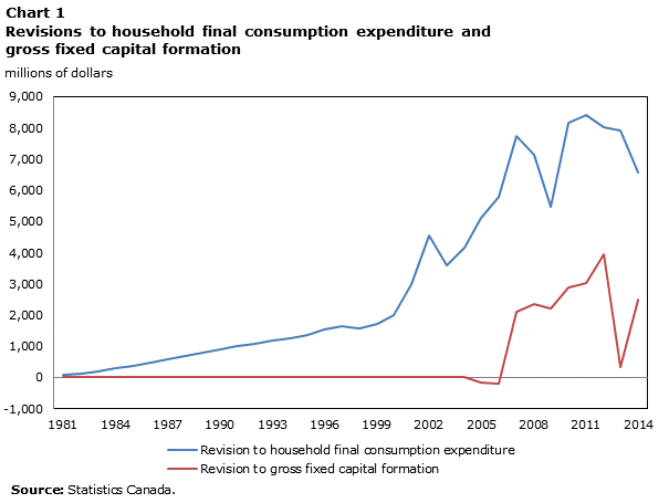
Description for Chart 1
The title of the graph is "Chart 1 Revisions to household final consumption expenditure and gross fixed capital formation."
This is a line chart.
There are in total 34 categories in the horizontal axis. The vertical axis starts at -1,000 and ends at 9,000 with ticks every 1,000 points.
There are 2 series in this graph.
The vertical axis is "millions of dollars."
The units of the horizontal axis are years from 1981 to 2014.
The title of series 1 is "Revision to household final consumption expenditure."
The minimum value is 72 occurring in 1981.
The maximum value is 8,411 occurring in 2011.
The title of series 2 is "Revision to gross fixed capital formation."
The minimum value is -215 occurring in 2006.
The maximum value is 3,958 occurring in 2012.
| Revision to household final consumption expenditure | Revision to gross fixed capital formation | |
|---|---|---|
| 1981 | 72 | -2 |
| 1982 | 116 | -2 |
| 1983 | 197 | -2 |
| 1984 | 291 | -3 |
| 1985 | 385 | -4 |
| 1986 | 472 | -2 |
| 1987 | 598 | 1 |
| 1988 | 700 | 2 |
| 1989 | 809 | 1 |
| 1990 | 913 | 0 |
| 1991 | 996 | 0 |
| 1992 | 1,076 | -1 |
| 1993 | 1,183 | -1 |
| 1994 | 1,245 | 1 |
| 1995 | 1,343 | 0 |
| 1996 | 1,530 | -2 |
| 1997 | 1,660 | -1 |
| 1998 | 1,589 | -1 |
| 1999 | 1,716 | -2 |
| 2000 | 2,008 | 1 |
| 2001 | 3,007 | 5 |
| 2002 | 4,547 | 5 |
| 2003 | 3,607 | 4 |
| 2004 | 4,175 | 4 |
| 2005 | 5,122 | -161 |
| 2006 | 5,802 | -215 |
| 2007 | 7,736 | 2,099 |
| 2008 | 7,156 | 2,365 |
| 2009 | 5,464 | 2,213 |
| 2010 | 8,180 | 2,899 |
| 2011 | 8,411 | 3,044 |
| 2012 | 8,010 | 3,958 |
| 2013 | 7,921 | 339 |
| 2014 | 6,566 | 2,504 |
| Source: Statistics Canada. | ||
There were also upward revisions in gross fixed capital formation – specifically investment in residential structures. A review of the methodology used to calculate the value of residential and non-residential structures determined that the value of taxes on production was being underrepresented. In particular, the value of land improvements transferred (or in-kind transfers) by developers to municipalities upon completion of residential subdivisions was being under-estimated. New source data obtained from government accounting records indicate that, on average, land developers’ transfer approximately 2.4 billion of in-kind taxes to municipal governments per year. This increased the value of construction investment.
3. Revisions to the growth in GDP
The revisions to the annual and quarterly growth in GDP over the entire revision period were minor. The mean absolute revision to the annual growth in nominal GDP was 0.13 percentage points between 1981 and 2014. Revisions were more substantial in the more recent periods. The mean absolute revision to annual nominal GDP for the period 2010 to 2014 was 0.2 percentage points.
Revisions to the growth in annual real GDP were similar. The mean absolute revision to the annual growth in real GDP was 0.11 percentage points between 1981 and 2014. The largest positive revision was in 2013, where annual real GDP was revised up 0.21 percentage points. The largest downward revision was in 2009, where annual real GDP was revised downward by 0.29 percentage points.
| Time period | Revised average growth in annual GDP (percent) | Previously published average growth in annual GDP (percent) | Mean absolute revision to the growth in annual GDP (percentage points) | Revised average growth in annual real GDP (percent) | Previously published average growth in annual real GDP (percent) | Mean absolute revision to the growth in annual real GDP (percentage points) |
|---|---|---|---|---|---|---|
| 1982 to 1989 | 7.80 | 7.79 | 0.13 | 2.88 | 2.90 | 0.14 |
| 1990 to 1999 | 4.16 | 4.16 | 0.08 | 2.37 | 2.38 | 0.08 |
| 2000 to 2009 | 4.62 | 4.63 | 0.14 | 2.08 | 2.09 | 0.10 |
| 2010 to 2014 | 4.72 | 4.74 | 0.20 | 2.53 | 2.54 | 0.18 |
| 1982 to 2014 | 5.27 | 5.27 | 0.13 | 2.43 | 2.44 | 0.11 |
| Source: Statistics Canada. | ||||||
Likewise, revisions to quarterly real GDP were minimal. There was no significant revision to the mean absolute revision to real quarterly GDP between 1981 and 2014. The largest positive revision was 0.32 in the first quarter of 1997 and the largest negative revision was 0.27 in the third quarter of 2014.
| Time period | Revised quarterly growth in real GDP (percent) | Previously published growth in real GDP (percent) | Revision (percentage points) | Mean absolute revision in real GDP (percentage points) |
|---|---|---|---|---|
| 1982 to 1989 | 0.66 | 0.66 | 0.00 | 0.07 |
| 1990 to 1999 | 0.63 | 0.64 | 0.00 | 0.08 |
| 2000 to 2009 | 0.48 | 0.49 | -0.01 | 0.09 |
| 2010 to 2014 | 0.58 | 0.57 | 0.01 | 0.14 |
| 1982 to 2014 | 0.60 | 0.60 | 0.00 | 0.09 |
| Source: Statistics Canada | ||||
The comprehensive revision did not change the business cycle over the period of the revision. The revised estimates continue to show a significant downturn in economic activity in 1981 to 1982, 1990 to 1991 and 2008 to 2009, as shown in charts 2, 3 and 4.
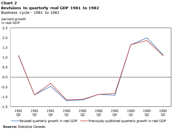
Description for Chart 2
The title of the graph is "Chart 2 Revisions to quarterly real GDP 1981 to 1982."
This is a line chart.
There are in total 10 categories in the horizontal axis. The vertical axis starts at -1.5 and ends at 2.5 with ticks every 0.5 points.
There are 2 series in this graph.
The vertical axis is "percent growth
in real GDP."
The units of the horizontal axis are quarters by year from second quarter 1981 to third quarter 1983.
The title of series 1 is "Revised quarterly growth in real GDP."
The minimum value is -1.19 occurring in first quarter 1982.
The maximum value is 1.99 occurring in second quarter 1983.
The title of series 2 is "Previously published quarterly growth in real GDP."
The minimum value is -1.15 occurring in first quarter 1982.
The maximum value is 1.87 occurring in second quarter 1983.
| Revised quarterly growth in real GDP | Previously published quarterly growth in real GDP | |
|---|---|---|
| 1981 | 1.10 | 1.08 |
| 1982 | -0.90 | -0.90 |
| 1983 | -0.46 | -0.31 |
| 1984 | -1.19 | -1.15 |
| 1985 | -1.15 | -1.12 |
| 1986 | -0.88 | -0.88 |
| 1987 | -0.92 | -0.83 |
| 1988 | 1.64 | 1.64 |
| 1989 | 1.99 | 1.87 |
| 1990 | 1.13 | 1.09 |
| Source: Statistics Canada. | ||
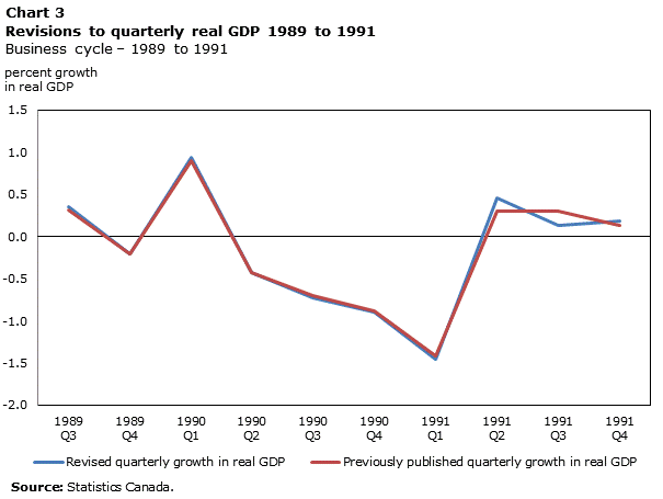
Description for Chart 3
The title of the graph is "Chart 3 Revisions to quarterly real GDP 1989 to 1991."
This is a line chart.
There are in total 10 categories in the horizontal axis. The vertical axis starts at -2 and ends at 1.5 with ticks every 0.5 points.
There are 2 series in this graph.
The vertical axis is "percent growth
in real GDP."
The units of the horizontal axis are quarters by year from third quarter 1989 to fourth quarter 1991.
The title of series 1 is "Revised quarterly growth in real GDP."
The minimum value is -1.45 occurring in first quarter 1991.
The maximum value is 0.94 occurring in first quarter 1990.
The title of series 2 is "Previously published quarterly growth in real GDP."
The minimum value is -1.41 occurring in first quarter 1991.
The maximum value is 0.9 occurring in first quarter 1990.
| Revised quarterly growth in real GDP | Previously published quarterly growth in real GDP | |
|---|---|---|
| 1989 | 0.36 | 0.32 |
| 1990 | -0.21 | -0.21 |
| 1991 | 0.94 | 0.90 |
| 1992 | -0.42 | -0.42 |
| 1993 | -0.72 | -0.70 |
| 1994 | -0.90 | -0.88 |
| 1995 | -1.45 | -1.41 |
| 1996 | 0.46 | 0.30 |
| 1997 | 0.13 | 0.30 |
| 1998 | 0.18 | 0.13 |
| Source: Statistics Canada. | ||
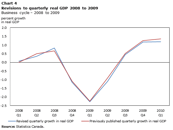
Description for Chart 4
The title of the graph is "Chart 4 Revisions to quarterly real GDP 2008 to 2009."
This is a line chart.
There are in total 9 categories in the horizontal axis. The vertical axis starts at -2.5 and ends at 2 with ticks every 0.5 points.
There are 2 series in this graph.
The vertical axis is "percent growth
in real GDP."
The units of the horizontal axis are quarters by year from first quarter 2008 to first quarter 2010.
The title of series 1 is "Revised quarterly growth in real GDP."
The minimum value is -2.28 occurring in first quarter 2009.
The maximum value is 1.19 occurring in first quarter 2010.
The title of series 2 is "Previously published quarterly growth in real GDP."
The minimum value is -2.25 occurring in first quarter 2009.
The maximum value is 1.36 occurring in first quarter 2010.
| Revised quarterly growth in real GDP | Previously published quarterly growth in real GDP | |
|---|---|---|
| 2008 | 0.06 | 0.00 |
| 2009 | 0.35 | 0.50 |
| 2010 | 0.83 | 0.66 |
| 2011 | -1.16 | -1.09 |
| 2012 | -2.28 | -2.25 |
| 2013 | -1.10 | -0.90 |
| 2014 | 0.45 | 0.52 |
| 2015 | 1.18 | 1.26 |
| 2016 | 1.19 | 1.36 |
| Source: Statistics Canada. | ||
4. Revisions to income-based GDP components
All income-based GDP components were revised as part of the 2015 comprehensive revision.
Revisions to compensation of employees
The major revision to compensation of employees was attributable to a revised treatment of defined benefit pension plans. Defined benefit pension plans are pension schemes that provide participants with a guaranteed future income stream upon retirement based on a formula (for example, a percentage of pay and years of service formula).
Pensions are contractual obligations between employers and employees. The contract entitles the employee to receive, as part of their compensation, a contribution to a pension plan made on their behalf by their employer. In theory, the contribution received by the employee should equal, in each accounting period, the amount they are entitled to as per the contractual obligation. For defined benefit plans, the entitlement represents the present value of future pension benefits. In practice, for a given period, the contributions of businesses and governments do not always match the entitlements of the employee. Sometimes contributions are less then entitlements, indicating that employers are underfunding the pension, and sometimes they are more, indicating that employers are overfunding the pension or attempting to reduce the underfunding of previous periods. The 2008 System of National Accounts recommends that the pension contributions be recorded as compensation of employees (employer social contributions) and that they reflect the entitlement accruing to the employee during the accounting period, rather than the cash contribution made by employers.
The previous treatment of pensions in the CSMA led to distortions in the compensation of employees series. For example, in Nova Scotia in 2011, the Government of Nova Scotia made large payment to the Nova Scotia Public Service Pension Plan. This payment reflected a ‘catch-up’ payment made by the government to ensure that the pension plan was properly funded to meet its future obligations. This resulted in a 23.9% increase in the employer social contributions in the province of Nova Scotia for the year 2011. The 23.9% did not represent an economic increase in the employer social contributions for 2011 but rather reflected an accumulation of past payments of employer social contributions that should have been recorded in previous years. The new treatment of pensions in the CSMA removes these distortions and places the payment in the period it was earned or entitled.
Recording pensions on an entitlement basis brings a number of important improvements to the national accounts. First, it aligns the timing of the flow of compensation of employees with the actual production of goods and services occurring during the accounting period. Second, it ensures that in each period the full pension assets and liabilities (the actuarial asset or liability) are recorded on each of the balance sheets of governments, trusteed pension plans, non-financial corporations and households, rather than the cash value of the accumulated asset or liability adjusted for market value. This ensures that the saving and consumption behaviours of governments and households are consistent with the stock of pension assets and liabilities on their respective balance sheets.
The recording of pension entitlements (pensions on an accrual basis) has resulted in revised estimates of employer social contributions for the period 1990 to 2015. Revisions were not carried back prior to 1990, as it was determined that the actual contributions were a good approximation of the entitlements for the period 1981 to 1990. Chart 5 compares the revised employer social contributions with the previously published employers’ social contributions. The revisions served to smooth out the series for the period open to revision. The total value of pension contributions over the period on the old basis was $595 billion while the total value of pension entitlements over the same period is $627 billion.
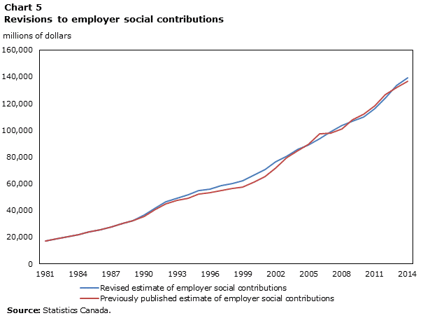
Description for Chart 5
The title of the graph is "Chart 5 Revisions to employer social contributions."
This is a line chart.
There are in total 34 categories in the horizontal axis. The vertical axis starts at 0 and ends at 160,000 with ticks every 20,000 points.
There are 2 series in this graph.
The vertical axis is "millions of dollars."
The units of the horizontal axis are years from 1981 to 2014.
The title of series 1 is "Revised estimate of employer social contributions."
The minimum value is 17,083 occurring in 1981.
The maximum value is 139,102 occurring in 2014.
The title of series 2 is "Previously published estimate of employer social contributions."
The minimum value is 17,083 occurring in 1981.
The maximum value is 136,397 occurring in 2014.
| Revised estimate of employer social contributions | Previously published estimate of employer social contributions | |
|---|---|---|
| 1981 | 17,083 | 17,083 |
| 1982 | 18,476 | 18,476 |
| 1983 | 20,204 | 20,204 |
| 1984 | 21,962 | 21,962 |
| 1985 | 23,996 | 23,996 |
| 1986 | 25,411 | 25,411 |
| 1987 | 27,685 | 27,685 |
| 1988 | 30,409 | 30,409 |
| 1989 | 32,026 | 32,026 |
| 1990 | 36,409 | 35,432 |
| 1991 | 41,883 | 40,568 |
| 1992 | 46,534 | 44,719 |
| 1993 | 49,248 | 47,580 |
| 1994 | 51,579 | 48,991 |
| 1995 | 54,599 | 52,433 |
| 1996 | 55,889 | 53,071 |
| 1997 | 58,318 | 55,036 |
| 1998 | 59,805 | 56,144 |
| 1999 | 62,029 | 57,343 |
| 2000 | 66,445 | 61,342 |
| 2001 | 70,470 | 65,243 |
| 2002 | 76,338 | 71,740 |
| 2003 | 80,610 | 79,262 |
| 2004 | 85,518 | 84,762 |
| 2005 | 88,816 | 89,373 |
| 2006 | 93,504 | 97,469 |
| 2007 | 98,949 | 97,640 |
| 2008 | 103,558 | 100,772 |
| 2009 | 106,901 | 107,811 |
| 2010 | 110,067 | 111,759 |
| 2011 | 116,375 | 118,459 |
| 2012 | 123,764 | 126,540 |
| 2013 | 133,362 | 131,983 |
| 2014 | 139,102 | 136,397 |
| Source: Statistics Canada. | ||
Revisions to gross operating surplus
Revisions to gross operating surplus were relatively small for the period 1981 to 2005 and larger for the period 2006 to 2015. The majority of the revisions for the 2010 to 2014 period reflect the incorporation of benchmark information from annual business survey’s and updated administrative data records.
| Time period | Revised estimate of gross operating surplus - non-financial corporations | Previously published estimate of gross operating surplus - non-financial corporations | Average revision to gross operating surplus - non-financial corporations |
|---|---|---|---|
| millions of dollars | |||
| 1981 to 1989 | 108,874 | 105,755 | 3,118 |
| 1990 to 1999 | 157,751 | 153,784 | 3,967 |
| 2000 to 2009 | 308,256 | 305,937 | 2,319 |
| 2010 to 2014 | 398,749 | 408,924 | -10,175 |
| Source: Statistics Canada. | |||
General government gross operating surplus, which reflects the consumption of fixed capital of the general government sector, was revised down with the 2015 comprehensive revision. The downward revision reflects changes in the service lives associated with the stock of government capital, as well as an improved methodology to estimate the consumption of fixed capital by sector. It was established that the asset services lives previously used in the CSMA were too high for non-residential buildings and structures, resulting in a lower value of the consumption of fixed capital. The revised services lives were calculated using a rich set of data constructed from over 10 years of responses to Statistics Canada’s Capital Expenditure and Repair Survey. The Capital Expenditure and Repair Survey collects information on the life of assets (both expected and actual). Estimates of service lives and depreciation profiles by asset are constructed from this information. These new service-lives data indicate that the stock of general government capital should have been consumed at a faster pace than previously estimated, increasing the consumption of fixed capital in the general government sector.
This service-lives increase was more than offset by a downward revision in the consumption of fixed capital due to an improvement in the way the capital stock is estimated by sector. With the improved capital stock estimates released in November 2014, there was a downward revision in the overall stock of capital estimated for the general government sector. This served to reduce the general government consumption of fixed capital over the revision period.
The combined result of the upward revision due to revised services lives and downward revision due to a revised capital stock is a small overall downward revision to total general government consumption of fixed capital, as shown in Table 5. Similarly, estimates of consumption of fixed capital for the non-profit institutions serving households’ sector was also revised down.
| Time period | Revised estimate of consumption of fixed capital - general government | Previously published estimate of consumption of fixed capital - general government | Revision to the estimate of consumption of fixed capital - general government |
|---|---|---|---|
| millions of dollars | |||
| 1981 to 1989 | 14,683 | 14,447 | 236 |
| 1990 to 1999 | 22,867 | 23,384 | -517 |
| 2000 to 2009 | 36,662 | 37,628 | -966 |
| 2010 to 2014 | 58,735 | 60,151 | -1,416 |
| Source: Statistics Canada. | |||
Revisions to taxes less subsidies on products and imports and taxes less subsidies on production
There were substantial revisions to taxes on production, due to the incorporation of improved government finance statistics. These revisions, like the revisions to general government final consumption expenditures, are due to the availability of new data sources, allowing for an improved delineation of taxes and subsidies.
As discussed previously, since 2007, the value of lot levies in-kind had been understated in the CSMA. Lot levies are classified as taxes on production in the CSMA. Lot levies in-kind represent the transfer of land improvements and structures by developers to municipalities upon the completion of development activities. An example is when a land developer develops a park within a sub-division and then transfers the land improvements associated with the park to the local municipality. The municipality accepts the land improvements in lieu of taxes. Chart 6 outlines the revisions to taxes on production—approximately half this revision is due to the treatment of lot levies in-kind. In addition to the lot levies revision, property taxes were also revised upward, essentially starting in 2011. The incorporation of the new government data provided a new, higher quality estimate of property taxes, resulting in an overall upward revision to taxes on production.
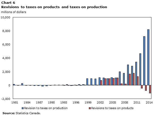
Description for Chart 6
The title of the graph is "Chart 6 Revisions to taxes on products and taxes on production."
This is a column clustered chart.
There are in total 34 categories in the horizontal axis. The vertical axis starts at -2,000 and ends at 10,000 with ticks every 2,000 points.
There are 2 series in this graph.
The vertical axis is "millions of dollars."
The units of the horizontal axis are years from 1981 to 2014.
The title of series 1 is "Revision to taxes on production."
The minimum value is -144 occurring in 1988.
The maximum value is 8,213 occurring in 2014.
The title of series 2 is "Revisions to taxes on products."
The minimum value is -1,176 occurring in 2014.
The maximum value is 1,772 occurring in 2010.
| Revision to taxes on production | Revisions to taxes on products | |
|---|---|---|
| 1981 | 149 | 0 |
| 1982 | -13 | 0 |
| 1983 | 267 | 0 |
| 1984 | -6 | 0 |
| 1985 | -5 | 0 |
| 1986 | -65 | 0 |
| 1987 | -66 | 0 |
| 1988 | -144 | 0 |
| 1989 | -90 | 0 |
| 1990 | -13 | 0 |
| 1991 | 43 | 0 |
| 1992 | 24 | 0 |
| 1993 | 35 | -3 |
| 1994 | 117 | -1 |
| 1995 | -51 | -2 |
| 1996 | 20 | -10 |
| 1997 | 106 | -1 |
| 1998 | 131 | 31 |
| 1999 | 1,005 | 47 |
| 2000 | 984 | 49 |
| 2001 | 964 | 48 |
| 2002 | 1,137 | 715 |
| 2003 | 1,083 | 978 |
| 2004 | 970 | 983 |
| 2005 | 1,155 | 1,030 |
| 2006 | 1,096 | 1,094 |
| 2007 | 2,012 | 237 |
| 2008 | 1,781 | 189 |
| 2009 | 3,017 | 1,676 |
| 2010 | 2,848 | 1,772 |
| 2011 | 3,429 | 1,275 |
| 2012 | 4,689 | -437 |
| 2013 | 7,184 | -775 |
| 2014 | 8,213 | -1,176 |
| Source: Statistics Canada. | ||
Similarly, there was an increase in the value of subsidies on production. A significant portion of the upward revision was due to the reclassification of subsidies related to crop insurance provided to farmers. Previously these were classified as subsidies on products. A review determined that these transactions better reflect subsidies on production, given they influence the production of the crop and are directed at farmers rather than levied on the sales directed towards consumers. As a result, subsidies on production were revised upward and subsidies on products were revised downwards as shown in Chart 7. The revisions to subsidies were also reflected in the gross operating surplus of corporations.
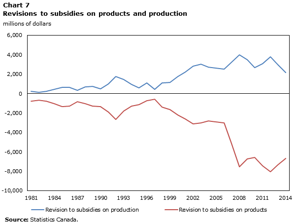
Description for Chart 7
The title of the graph is "Chart 7 Revisions to subsidies on products and production."
This is a line chart.
There are in total 34 categories in the horizontal axis. The vertical axis starts at -10,000 and ends at 6,000 with ticks every 2,000 points.
There are 2 series in this graph.
The vertical axis is "millions of dollars."
The units of the horizontal axis are years from 1981 to 2014.
The title of series 1 is "Revision to subsidies on production."
The minimum value is 113 occurring in 1982.
The maximum value is 3,975 occurring in 2008.
The title of series 2 is "Revision to subsidies on products."
The minimum value is -8,055 occurring in 2012.
The maximum value is -601 occurring in 1997.
| Revision to subsidies on production | Revision to subsidies on products | |
|---|---|---|
| 1981 | 230 | -785 |
| 1982 | 113 | -671 |
| 1983 | 238 | -772 |
| 1984 | 432 | -1,020 |
| 1985 | 641 | -1,325 |
| 1986 | 656 | -1,279 |
| 1987 | 328 | -822 |
| 1988 | 690 | -1,041 |
| 1989 | 760 | -1,277 |
| 1990 | 505 | -1,348 |
| 1991 | 972 | -1,900 |
| 1992 | 1,776 | -2,646 |
| 1993 | 1,465 | -1,808 |
| 1994 | 965 | -1,290 |
| 1995 | 579 | -1,136 |
| 1996 | 1,092 | -738 |
| 1997 | 452 | -601 |
| 1998 | 1,109 | -1,400 |
| 1999 | 1,139 | -1,621 |
| 2000 | 1,742 | -2,181 |
| 2001 | 2,229 | -2,599 |
| 2002 | 2,817 | -3,104 |
| 2003 | 3,044 | -3,030 |
| 2004 | 2,701 | -2,793 |
| 2005 | 2,616 | -2,903 |
| 2006 | 2,511 | -3,041 |
| 2007 | 3,211 | -5,160 |
| 2008 | 3,975 | -7,517 |
| 2009 | 3,466 | -6,714 |
| 2010 | 2,657 | -6,572 |
| 2011 | 3,066 | -7,424 |
| 2012 | 3,783 | -8,055 |
| 2013 | 2,979 | -7,323 |
| 2014 | 2,159 | -6,680 |
| Source: Statistics Canada. | ||
5. Revisions to expenditure-based GDP components
The majority of expenditure-based GDP components were revised with the 2015 comprehensive revision.
General government final consumption expenditure
As noted, government final consumption expenditure was revised significantly for the period 2010 to 2014. Revisions occurred for all levels of government and all major components of final consumption expenditure (consumption of fixed capital, compensation of employees and other non-wage expenditures). Total general government final consumption expenditure was revised down by an average of $9.9 billion per year between 2010 and 2014. Although compensation of employees was revised upwards, it was more than offset by downward revisions in consumption of fixed capital and other non-wage components.
| Time period | Current general government final consumption expenditure | Previously published general government final consumption expenditure | Total revision | Revision to general government compensation of employees | Revision to general government consumption of fixed capital | Revision to general government, other non-wage |
|---|---|---|---|---|---|---|
| millions of dollars | ||||||
| 1981 to 1989 | 110,142 | 108,762 | 1,380 | 0 | 0 | 0 |
| 1990 to 1999 | 177,949 | 177,020 | 930 | 0 | 0 | 0 |
| 2000 to 2009 | 271,458 | 271,531 | -73 | 2,016 | -441 | -2,761 |
| 2010 to 2014 | 384,335 | 394,183 | -9,848 | 7,792 | -1,416 | -15,118 |
| Source: Statistics Canada. | ||||||
Revisions were concentrated in the local government sub-sector. On average, local general government final consumption expenditure was revised down by $5.5 billion for the period 2010 to 2014. The downward revision is a result of updated data for local governments incorporated into the CSMA. Previously, data were estimated from incomplete local general government documents and often reflected budgetary information. The revised estimates now align with the actual spending by local general governments and incorporate the latest available information from public accounting statements. Revisions to final consumption expenditure for federal and provincial or territorial governments were smaller than local governments. Federal government revisions mainly reflect changes in the treatment of employer pensions; whereas revisions to the provincial and territorial government reflect new estimates compiled directly from provincial and territorial general ledgers. This improved data source permits a better estimate of provincial and territorial general government final consumption expenditures.
| Time period | Average current general government final consumption expenditure | Average previously published general government final consumption expenditure | Average total revision | Average revision to federal general government final consumption expenditure | Average revision to provincial and territorial general government final consumption expenditure | Average revision to local general government final consumption expenditure | Average revision to Aboriginal general government final consumption expenditure |
|---|---|---|---|---|---|---|---|
| millions of dollars | |||||||
| 1981 to 1989 | 110,142 | 108,762 | 1,380 | 357 | 1,080 | -190 | 134 |
| 1990 to 1999 | 177,949 | 177,020 | 930 | 433 | 552 | 11 | -64 |
| 2000 to 2009 | 271,458 | 271,531 | -73 | 438 | 1,264 | -1,538 | -419 |
| 2010 to 2014 | 384,335 | 394,183 | -9,848 | -1,070 | -3,568 | -5,588 | -609 |
| Total period | 217,854 | 218,685 | -831 | 193 | 295 | -1,321 | -196 |
| Source: Statistics Canada. | |||||||
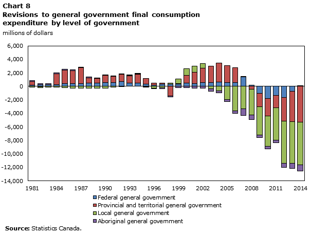
Description for Chart 8
The title of the graph is "Chart 8 Revisions to general government final consumption expenditure by level of government."
This is a column stacked chart.
There are in total 34 categories in the horizontal axis. The vertical axis starts at -14,000 and ends at 6,000 with ticks every 2,000 points.
There are 4 series in this graph.
The vertical axis is "millions of dollars."
The units of the horizontal axis are years from 1981 to 2014.
The title of series 1 is "Federal general government."
The minimum value is -1,806 occurring in 2010.
The maximum value is 1,430 occurring in 2007.
The title of series 2 is "Provincial and territorial general government."
The minimum value is -5,275 occurring in 2014.
The maximum value is 2,788 occurring in 2004.
The title of series 3 is "Local general government."
The minimum value is -6,323 occurring in 2014.
The maximum value is 963 occurring in 2000.
The title of series 4 is "Aboriginal general government."
The minimum value is -984 occurring in 2007.
The maximum value is 169 occurring in 1982.
| Federal general government | Provincial and territorial general government | Local general government | Aboriginal general government | |
|---|---|---|---|---|
| 1981 | 182 | 506 | -89 | 159 |
| 1982 | 270 | -73 | -107 | 169 |
| 1983 | 239 | 50 | -133 | 158 |
| 1984 | 293 | 1,561 | -147 | 145 |
| 1985 | 400 | 1,964 | -202 | 147 |
| 1986 | 424 | 1,925 | -245 | 109 |
| 1987 | 445 | 2,319 | -250 | 113 |
| 1988 | 467 | 793 | -267 | 106 |
| 1989 | 496 | 674 | -271 | 101 |
| 1990 | 564 | 1,099 | -243 | 15 |
| 1991 | 556 | 929 | -87 | 9 |
| 1992 | 690 | 1,062 | -2 | 11 |
| 1993 | 453 | 1,120 | 56 | 10 |
| 1994 | 505 | 1,304 | 21 | 45 |
| 1995 | 369 | 837 | -37 | -80 |
| 1996 | 206 | 301 | -287 | -50 |
| 1997 | 328 | 178 | -216 | -166 |
| 1998 | 302 | -1,385 | 197 | -211 |
| 1999 | 352 | 74 | 703 | -223 |
| 2000 | 472 | 1,166 | 963 | -210 |
| 2001 | 409 | 1,642 | 927 | -245 |
| 2002 | 539 | 2,182 | 653 | -294 |
| 2003 | 580 | 2,445 | -368 | -329 |
| 2004 | 642 | 2,788 | -621 | -341 |
| 2005 | 537 | 2,528 | -1,922 | -354 |
| 2006 | 589 | 2,216 | -3,651 | -395 |
| 2007 | 1,430 | 38 | -3,296 | -984 |
| 2008 | 202 | -395 | -3,874 | -658 |
| 2009 | -1,017 | -1,969 | -4,187 | -383 |
| 2010 | -1,806 | -2,611 | -4,487 | -355 |
| 2011 | -1,339 | -1,835 | -4,810 | -341 |
| 2012 | -1,610 | -3,575 | -6,218 | -579 |
| 2013 | -720 | -4,545 | -6,102 | -830 |
| 2014 | 126 | -5,275 | -6,323 | -941 |
| Source: Statistics Canada. | ||||
Part of the revision to general government final consumption expenditure is attributable to an upward revision in the sale of government goods and services. Smaller revisions were recorded for the period 1981 to 2003 while more substantial revisions were incorporated for the period 2004 to 2014. Sales of goods and services of general governments include items such as the rental of recreational facilities and the purchase of permits.
The value of general government final consumption expenditure that is used in the calculation of expenditure-based gross domestic product is net of the sale of goods and services. For example, if the government spends $100 to deliver a service and receives $25 from a household in the form of a user fee then the ‘net’ general government final consumption expenditure is $75. This ‘netting’ is done to avoid double counting in the calculation of gross domestic product, since the sale of the government good or service is either a purchase by households (and therefore included in household final consumption expenditure) or intermediate consumption, purchased by businesses (and therefore a subtraction in the calculation of gross domestic product). An upward revision in the general governments’ sale of goods and services without a corresponding upward revision in household final consumption expenditures will result in a downward revision to gross domestic product. This is the case with this revision. In previously-published estimates the sales of the general government goods and services were properly reflected in the individual household final consumption expenditure series but not reflected in the general government final consumption expenditure. In addition, some of the upwardly revised sales of goods and services were sold to businesses. Both of these result in a downward revision to gross domestic product.
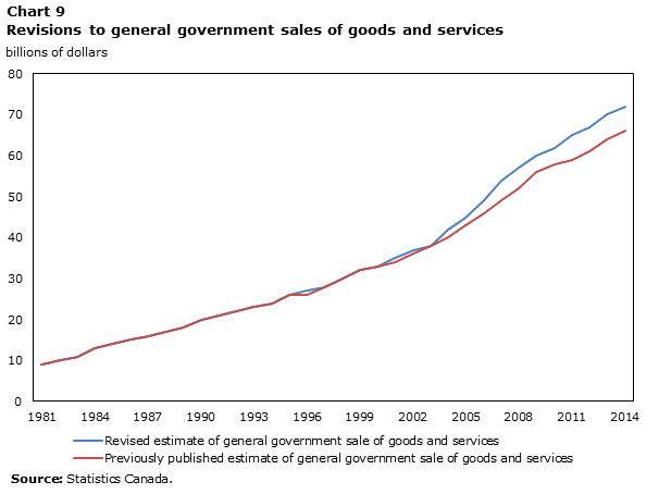
Description for Chart 9
The title of the graph is "Chart 9 Revisions to general government sales of goods and services."
This is a line chart.
There are in total 34 categories in the horizontal axis. The vertical axis starts at 0 and ends at 80 with ticks every 10 points.
There are 2 series in this graph.
The vertical axis is "billions of dollars."
The units of the horizontal axis are years from 1981 to 2014.
The title of series 1 is "Revised estimate of general government sale of goods and services."
The minimum value is 9 occurring in 1981.
The maximum value is 72 occurring in 2014.
The title of series 2 is "Previously published estimate of general government sale of goods and services."
The minimum value is 9 occurring in 1981.
The maximum value is 66 occurring in 2014.
| Revised estimate of general government sale of goods and services | Previously published estimate of general government sale of goods and services | |
|---|---|---|
| 1981 | 9 | 9 |
| 1982 | 10 | 10 |
| 1983 | 11 | 11 |
| 1984 | 13 | 13 |
| 1985 | 14 | 14 |
| 1986 | 15 | 15 |
| 1987 | 16 | 16 |
| 1988 | 17 | 17 |
| 1989 | 18 | 18 |
| 1990 | 20 | 20 |
| 1991 | 21 | 21 |
| 1992 | 22 | 22 |
| 1993 | 23 | 23 |
| 1994 | 24 | 24 |
| 1995 | 26 | 26 |
| 1996 | 27 | 26 |
| 1997 | 28 | 28 |
| 1998 | 30 | 30 |
| 1999 | 32 | 32 |
| 2000 | 33 | 33 |
| 2001 | 35 | 34 |
| 2002 | 37 | 36 |
| 2003 | 38 | 38 |
| 2004 | 42 | 40 |
| 2005 | 45 | 43 |
| 2006 | 49 | 46 |
| 2007 | 54 | 49 |
| 2008 | 57 | 52 |
| 2009 | 60 | 56 |
| 2010 | 62 | 58 |
| 2011 | 65 | 59 |
| 2012 | 67 | 61 |
| 2013 | 70 | 64 |
| 2014 | 72 | 66 |
| Source: Statistics Canada. | ||
Inventories
The improved granularity associated with the new GFS data permitted the estimation of new components of government inventories not possible with prior sources of information. In the past, all expenditures of government were recorded as current government final consumption expenditure, regardless of whether they were consumed in the accounting period or not. International standards recommend that government expenditure be recorded when the goods and services are consumed rather than when the material inputs are purchased. Given the detailed nature of the government data now available to construct Canada’s national accounts, it is possible to estimate the value of government investment in inventories, starting in 2007. Prior to that date, purchases held in inventory are recorded as government final consumption expenditure.
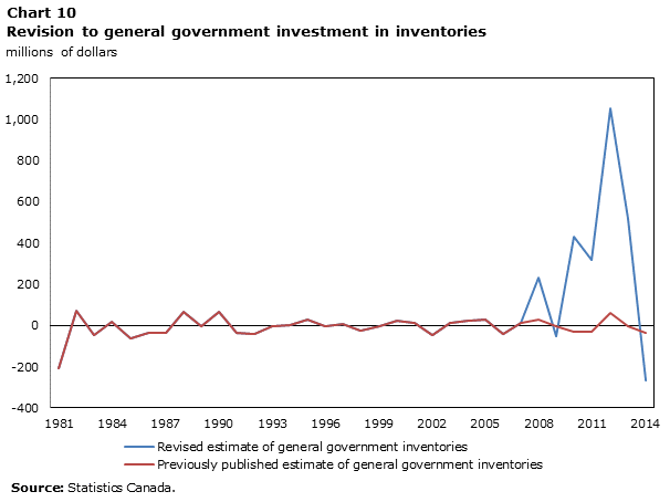
Description for Chart 10
The title of the graph is "Chart 10 Revision to general government investment in inventories."
This is a line chart.
There are in total 34 categories in the horizontal axis. The vertical axis starts at -400 and ends at 1,200 with ticks every 200 points.
There are 2 series in this graph.
The vertical axis is "millions of dollars."
The units of the horizontal axis are years from 1981 to 2014.
The title of series 1 is "Revised estimate of general government inventories."
The minimum value is -267 occurring in 2014.
The maximum value is 1,052 occurring in 2012.
The title of series 2 is "Previously published estimate of general government inventories."
The minimum value is -205 occurring in 1981.
The maximum value is 69 occurring in 1982.
| Revised estimate of general government inventories | Previously published estimate of general government inventories | |
|---|---|---|
| 1981 | -205 | -205 |
| 1982 | 69 | 69 |
| 1983 | -45 | -45 |
| 1984 | 20 | 20 |
| 1985 | -64 | -64 |
| 1986 | -35 | -35 |
| 1987 | -38 | -38 |
| 1988 | 64 | 64 |
| 1989 | -3 | -3 |
| 1990 | 67 | 67 |
| 1991 | -37 | -37 |
| 1992 | -40 | -40 |
| 1993 | -4 | -4 |
| 1994 | -1 | -1 |
| 1995 | 30 | 30 |
| 1996 | -2 | -2 |
| 1997 | 5 | 5 |
| 1998 | -27 | -27 |
| 1999 | -3 | -3 |
| 2000 | 24 | 24 |
| 2001 | 13 | 13 |
| 2002 | -45 | -45 |
| 2003 | 15 | 15 |
| 2004 | 21 | 21 |
| 2005 | 27 | 27 |
| 2006 | -41 | -41 |
| 2007 | 15 | 15 |
| 2008 | 231 | 29 |
| 2009 | -53 | -3 |
| 2010 | 432 | -31 |
| 2011 | 319 | -32 |
| 2012 | 1,052 | 59 |
| 2013 | 518 | -6 |
| 2014 | -267 | -36 |
| Source: Statistics Canada. | ||
Household final consumption expenditure
With the 2015 comprehensive revision, there were substantial upward revisions to household final consumption expenditure, mainly due to revised estimates of household purchases of financial services, specifically financial investment services, as described earlier. Revisions to other components were much smaller and mainly reflect the reclassification of transactions. For example, driver’s licence fees were previously classified as a tax and are now classified as household final consumption expenditure. Chart 11 provides a breakdown of the revision to household final consumption expenditure by durability class.
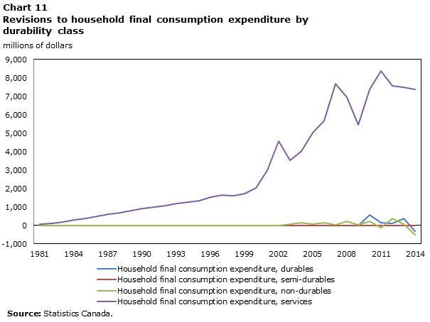
Description for Chart 11
The title of the graph is "Chart 11 Revisions to household final consumption expenditure by durability class."
This is a line chart.
There are in total 34 categories in the horizontal axis. The vertical axis starts at -1,000 and ends at 9,000 with ticks every 1,000 points.
There are 4 series in this graph.
The vertical axis is "millions of dollars."
The units of the horizontal axis are years from 1981 to 2014.
The title of series 1 is "Household final consumption expenditure, durables."
The minimum value is -308 occurring in 2014.
The maximum value is 575 occurring in 2010.
The title of series 2 is "Household final consumption expenditure, semi-durables."
The minimum value is -20 occurring in 2013.
The maximum value is 0 occurring in 1981, 1982, 1983, 1984, 1985, 1986, 1987, 1988, 1989, 1990, 1991, 1992, 1993, 1994, 1995, 1996, 1997, 1998, 1999, 2000, 2001, 2002, 2003, 2004, 2005, 2006, 2007, 2008, 2009, 2010 and 2011.
The title of series 3 is "Household final consumption expenditure, non-durables."
The minimum value is -514 occurring in 2014.
The maximum value is 362 occurring in 2012.
The title of series 4 is "Household final consumption expenditure, services."
The minimum value is 72 occurring in 1981.
The maximum value is 8,388 occurring in 2011.
| Household final consumption expenditure, durables | Household final consumption expenditure, semi-durables | Household final consumption expenditure, non-durables | Household final consumption expenditure, services | |
|---|---|---|---|---|
| 1981 | 0 | 0 | 0 | 72 |
| 1982 | 0 | 0 | 0 | 116 |
| 1983 | 0 | 0 | 0 | 197 |
| 1984 | 0 | 0 | 0 | 291 |
| 1985 | 0 | 0 | 0 | 385 |
| 1986 | 0 | 0 | 0 | 472 |
| 1987 | 0 | 0 | 0 | 598 |
| 1988 | 0 | 0 | 0 | 700 |
| 1989 | 0 | 0 | 0 | 809 |
| 1990 | 0 | 0 | -1 | 914 |
| 1991 | 0 | 0 | -2 | 998 |
| 1992 | 0 | 0 | -3 | 1,079 |
| 1993 | 0 | 0 | -4 | 1,187 |
| 1994 | 0 | 0 | -3 | 1,248 |
| 1995 | 0 | 0 | -4 | 1,347 |
| 1996 | 0 | 0 | -4 | 1,534 |
| 1997 | 0 | 0 | -4 | 1,664 |
| 1998 | 0 | 0 | -4 | 1,593 |
| 1999 | 0 | 0 | -4 | 1,720 |
| 2000 | 0 | 0 | -4 | 2,012 |
| 2001 | 0 | 0 | -4 | 3,011 |
| 2002 | 0 | 0 | -5 | 4,552 |
| 2003 | 0 | 0 | 60 | 3,547 |
| 2004 | 0 | 0 | 162 | 4,013 |
| 2005 | 0 | 0 | 74 | 5,048 |
| 2006 | 0 | 0 | 126 | 5,676 |
| 2007 | 0 | 0 | 30 | 7,706 |
| 2008 | 0 | 0 | 215 | 6,941 |
| 2009 | 0 | 0 | 25 | 5,439 |
| 2010 | 575 | 0 | 210 | 7,395 |
| 2011 | 132 | 0 | -109 | 8,388 |
| 2012 | 101 | -9 | 362 | 7,556 |
| 2013 | 359 | -20 | 73 | 7,509 |
| 2014 | -308 | -7 | -514 | 7,395 |
| Source: Statistics Canada. | ||||
Residential and non-residential investment
As noted, the CSMA previously underestimated the lot levies charged to land developers by municipalities. In a number of jurisdictions in Canada land developers provide assets, such as parks, to local governments in lieu of paying these land development fees. In the past, since their value was not known, these in-kind development fees were not included in the methodology used by Statistics Canada to determine the market price of residential investment. These in-kind lot levies—which represent a part of the basic price of a residential structure—have now been added to the value of construction investment. Data have been revised back to 2007, as it was determined that fees of this nature are insignificant prior to this time. Over the 8-year period the value of residential and non-residential investment was revised up by an average of $2.4 billion, residential investment, in particular, was revised $1.8 billion.
| Time period | Current estimate of investment in residential structures (business sector) | Previously published estimate of investment in residential structures (business sector) | Revision to investment in residential structures (business sector) |
|---|---|---|---|
| millions of dollars | |||
| 1981 to 1989 | 29,541 | 29,541 | 0 |
| 1990 to 1999 | 40,504 | 40,504 | 0 |
| 2000 to 2009 | 83,008 | 82,492 | 515 |
| 2010 to 2014 | 124,705 | 122,732 | 1,973 |
| Total period | 62,485 | 62,044 | 442 |
| Source: Statistics Canada. | |||
Exports and imports of goods and services
Revisions to exports and imports were minimal over the revision period. The majority occurred for the period 2010 and 2014 and were a result of the incorporation of new benchmark information available from the supply-use tables and the international merchandise trade statistics program.
6. Revisions to incomes, consumption, saving and net lending or borrowing by sector
Revisions to household incomes, consumption and saving due to changes in the treatment of pensions
There were revisions to household income, consumption and saving for the period 1981 to the present. The majority of the revisions to household income reflect the changes in the treatment of defined benefit pension plans. This served to smooth out the flows associated with pensions (contributions, investment income and withdrawals) to and from the household sector, resulting in both upward and downward revisions over the historical period.
As noted earlier, household pensions are now recorded on an entitlement (accrual) basis rather than on a cash basis in the CSMA. This means that the CSMA records the value of pension benefits accrued to them as part of their pension contract rather than the actual cash contributed in a given period. This new treatment results in four new flows in the household sector’s current and capital accounts. An example of these flows is depicted in Table 9.
The first flow represents the contribution made by the employer to the employee for the labour services provided during the accounting period. As noted earlier, this flow represents the contractual obligation of the employer to the employee and not the cash contribution. For example, suppose that, according to the contractual obligation, the employer was required to contribute $50 to the employee’s pension fund but only contributed $25. Within the CSMA the full $50 would be recorded. The CSMA would recognize the actual contribution of $25 as well as impute an additional $25 contribution as showing in Table 9.
The second flow relates to a corresponding accrual treatment with respect to the property income received by the household sector from the pension plan. As an example, assume an employer has entered into a contractual obligation with a group of employees and will pay them 50% of their latest year’s annual income upon retirement. Assume that, at the moment, the employer has not made any contributions to the pension plan and an actuarial assessment has determined that to meet contractual obligations there should be $50 million in the fund. Had the employer made the $50 million contribution, the funds would have been invested and earned investment income. This foregone property income is now imputed within the CSMA and recorded as a flow from the pension fund to the household sector. For the purposes of the example assume that this imputed flow of income is $5 and is represented in Table 9 as the receipt of property income by households from pension funds, recorded in the financial corporations’ sector.
The third flow reflects the household’s contributions to the pension plan. Employer contributions to pension plans on behalf of employees are first reflected in the CSMA as compensation of employees and recorded in the household sector. These funds are then transferred from the household sector to the pension fund. Similarly, the investment income earned on a pension fund is first recorded as earned by the household sector, since they are the ultimate owner of the asset. The sector then re-invests (or transfers) this investment income back into the pension fund. In the past, these flows were not explicitly identifiable because pension funds were part of the household sector. Pension funds are now shown in the financial corporations’ sector and the flows between the sectors are fully articulated. In the household sector table, these flows are recorded as current transfers to financial corporations. For the purposes of the example this represents a flow of $75 from the household sector to the financial corporation sector - $50 reflecting the contributions (actual and imputed) from the employer, $20 reflecting the employees contribution to their pension fund and $5 reflecting the reinvestment of property income earned.
The fourth new flow in the household sector’s current and capital account are related to pension benefits paid to pensioners. In the past, these flows were simply reflected as a drawing-down in the household sector’s pension assets and were only visible as a change in pension assets from one period to the next. With the 2015 CSMA revision, these contributions are recorded as current transfers received by households from financial corporations. Assume, for the purposes of the example that $20 was withdrawn from pension funds in the accounting period.
The final flow added to the household sector’s current and capital account is the ‘change in pension entitlements’. This flow is required to ensure that the entire pension asset (including the unfunded portion) is recorded in the household sector. It represents the difference between pension withdrawals and pension contributions and investment income transferred from the household to the pension fund. This is reflected in the $55 in change in pension entitlements in Table 9.
| Flow | Non-financial corporations sector | Household sector | Financial corporations sector |
|---|---|---|---|
| Actual employer social contributions | -25 | +25 | This is an empty cell |
| Imputed employer social contributions | -25 | +25 | This is an empty cell |
| Property income received | This is an empty cell | +5 | -5 |
| Current transfers (pension contributions) | This is an empty cell | -75 | 75 |
| Current transfers (pension withdrawals) | This is an empty cell | +20 | -20 |
| Household disposable income | This is an empty cell | -55 | This is an empty cell |
| Change in pension entitlements | This is an empty cell | 55 | -55 |
| Source: Statistics Canada. | |||
Given that the household sector’s contributions to pensions have been larger than their withdrawals over the period of the revision and the new flow – change in pension entitlements is added after the calculation of household disposable income – household disposable income was revised downward as shown in Chart 12.
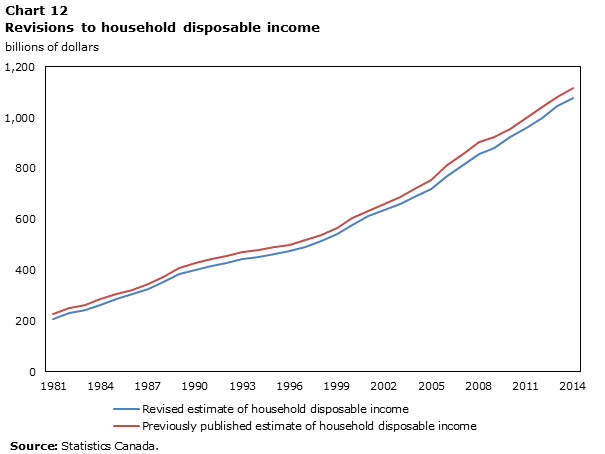
Description for Chart 12
The title of the graph is "Chart 12 Revisions to household disposable income."
This is a line chart.
There are in total 34 categories in the horizontal axis. The vertical axis starts at 0 and ends at 1,200 with ticks every 200 points.
There are 2 series in this graph.
The vertical axis is "billions of dollars."
The units of the horizontal axis are years from 1981 to 2014.
The title of series 1 is "Revised estimate of household disposable income."
The minimum value is 209 occurring in 1981.
The maximum value is 1,076 occurring in 2014.
The title of series 2 is "Previously published estimate of household disposable income."
The minimum value is 225 occurring in 1981.
The maximum value is 1,118 occurring in 2014.
| Revised estimate of household disposable income | Previously published estimate of household disposable income | |
|---|---|---|
| 1981 | 209 | 225 |
| 1982 | 230 | 249 |
| 1983 | 242 | 261 |
| 1984 | 263 | 284 |
| 1985 | 287 | 307 |
| 1986 | 304 | 323 |
| 1987 | 324 | 343 |
| 1988 | 353 | 374 |
| 1989 | 385 | 406 |
| 1990 | 401 | 426 |
| 1991 | 416 | 442 |
| 1992 | 429 | 455 |
| 1993 | 444 | 471 |
| 1994 | 452 | 478 |
| 1995 | 463 | 491 |
| 1996 | 473 | 499 |
| 1997 | 492 | 517 |
| 1998 | 515 | 539 |
| 1999 | 543 | 567 |
| 2000 | 576 | 605 |
| 2001 | 611 | 631 |
| 2002 | 638 | 660 |
| 2003 | 659 | 687 |
| 2004 | 691 | 722 |
| 2005 | 717 | 756 |
| 2006 | 770 | 814 |
| 2007 | 812 | 857 |
| 2008 | 858 | 904 |
| 2009 | 881 | 922 |
| 2010 | 924 | 956 |
| 2011 | 958 | 1,000 |
| 2012 | 997 | 1,041 |
| 2013 | 1,044 | 1,081 |
| 2014 | 1,076 | 1,118 |
| Source: Statistics Canada. | ||
Revision to the household saving rate
As mentioned, household consumption was revised up. This increase in consumption was smaller than the upward revision to household disposable income (including the change in pension entitlements) and therefore household saving was generally revised upward, with larger revisions recorded in the 1981 to 2003 time period. The household saving rate (household saving divided by household disposable income) was revised from an average of 7.7% to 8.3% between 1981 and 2014.
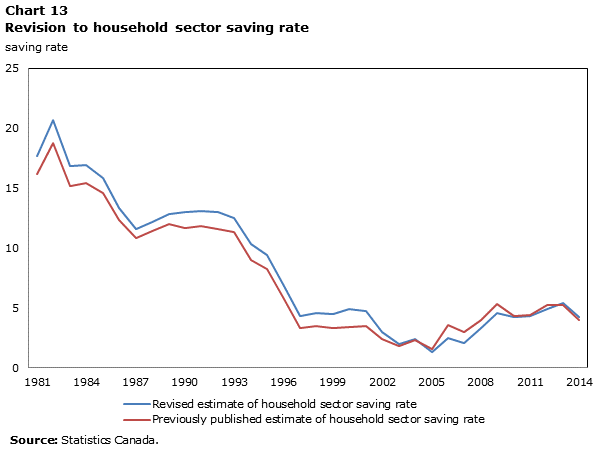
Description for Chart 13
The title of the graph is "Chart 13 Revision to household sector saving rate."
This is a line chart.
There are in total 34 categories in the horizontal axis. The vertical axis starts at 0 and ends at 25 with ticks every 5 points.
There are 2 series in this graph.
The vertical axis is "saving rate."
The units of the horizontal axis are years from 1981 to 2014.
The title of series 1 is "Revised estimate of household sector saving rate."
The minimum value is 1.3 occurring in 2005.
The maximum value is 20.7 occurring in 1982.
The title of series 2 is "Previously published estimate of household sector saving rate."
The minimum value is 1.6 occurring in 2005.
The maximum value is 18.8 occurring in 1982.
| Revised estimate of household sector saving rate | Previously published estimate of household sector saving rate | |
|---|---|---|
| 1981 | 17.7 | 16.2 |
| 1982 | 20.7 | 18.8 |
| 1983 | 16.8 | 15.2 |
| 1984 | 16.9 | 15.4 |
| 1985 | 15.8 | 14.6 |
| 1986 | 13.3 | 12.3 |
| 1987 | 11.6 | 10.8 |
| 1988 | 12.2 | 11.4 |
| 1989 | 12.8 | 12.0 |
| 1990 | 13.0 | 11.7 |
| 1991 | 13.1 | 11.8 |
| 1992 | 13.0 | 11.6 |
| 1993 | 12.5 | 11.3 |
| 1994 | 10.3 | 9.0 |
| 1995 | 9.4 | 8.2 |
| 1996 | 6.8 | 5.7 |
| 1997 | 4.3 | 3.3 |
| 1998 | 4.6 | 3.5 |
| 1999 | 4.5 | 3.3 |
| 2000 | 4.9 | 3.4 |
| 2001 | 4.7 | 3.5 |
| 2002 | 3.0 | 2.4 |
| 2003 | 2.0 | 1.8 |
| 2004 | 2.4 | 2.3 |
| 2005 | 1.3 | 1.6 |
| 2006 | 2.5 | 3.6 |
| 2007 | 2.1 | 3.0 |
| 2008 | 3.3 | 4.0 |
| 2009 | 4.6 | 5.3 |
| 2010 | 4.2 | 4.3 |
| 2011 | 4.3 | 4.4 |
| 2012 | 4.9 | 5.2 |
| 2013 | 5.4 | 5.2 |
| 2014 | 4.2 | 4.0 |
| Source: Statistics Canada. | ||
This revision to the household sector did little to change the sectors’ net lending or borrowing position. As illustrated in the following chart, in 1996, households moved from a net lending to a net borrowing position, which meant that the savings households generated were no longer sufficient to meet their demand for funds to invest in non-financial assets, such as residential structures. This position remains unchanged. Chart 14 compares the current and previously published net borrowing position of households.
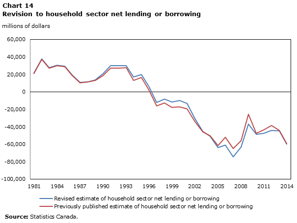
Description for Chart 14
The title of the graph is "Chart 14 Revision to household sector net lending or borrowing."
This is a line chart.
There are in total 34 categories in the horizontal axis. The vertical axis starts at -100,000 and ends at 60,000 with ticks every 20,000 points.
There are 2 series in this graph.
The vertical axis is "millions of dollars."
The units of the horizontal axis are years from 1981 to 2014.
The title of series 1 is "Revised estimate of household sector net lending or borrowing."
The minimum value is -74,622 occurring in 2007.
The maximum value is 37,979 occurring in 1982.
The title of series 2 is "Previously published estimate of household sector net lending or borrowing."
The minimum value is -64,877 occurring in 2007.
The maximum value is 37,237 occurring in 1982.
| Revised estimate of household sector net lending or borrowing | Previously published estimate of household sector net lending or borrowing | |
|---|---|---|
| 1981 | 21,540 | 20,902 |
| 1982 | 37,979 | 37,237 |
| 1983 | 27,839 | 27,062 |
| 1984 | 30,419 | 29,727 |
| 1985 | 29,325 | 28,857 |
| 1986 | 19,087 | 18,615 |
| 1987 | 10,756 | 10,340 |
| 1988 | 11,573 | 11,178 |
| 1989 | 13,604 | 13,245 |
| 1990 | 21,123 | 18,829 |
| 1991 | 29,818 | 27,389 |
| 1992 | 30,169 | 27,104 |
| 1993 | 30,066 | 27,517 |
| 1994 | 16,933 | 13,341 |
| 1995 | 19,634 | 16,361 |
| 1996 | 6,339 | 2,631 |
| 1997 | -11,984 | -16,097 |
| 1998 | -8,063 | -12,765 |
| 1999 | -11,787 | -17,541 |
| 2000 | -10,105 | -17,301 |
| 2001 | -13,083 | -19,492 |
| 2002 | -30,436 | -33,962 |
| 2003 | -45,051 | -45,638 |
| 2004 | -50,685 | -50,332 |
| 2005 | -63,612 | -61,300 |
| 2006 | -61,087 | -51,768 |
| 2007 | -74,622 | -64,877 |
| 2008 | -63,307 | -55,877 |
| 2009 | -37,039 | -25,380 |
| 2010 | -48,637 | -47,722 |
| 2011 | -47,553 | -43,621 |
| 2012 | -44,217 | -38,731 |
| 2013 | -44,491 | -44,426 |
| 2014 | -59,946 | -59,551 |
| Source: Statistics Canada. | ||
Revisions to the net lending or borrowing of governments
The net lending or borrowing positions of general governments were revised substantially over the revision period—specifically in the 2007 to 2014 period. On average, between 2007 and 2014 the general governments borrowed less than was previously estimated. This revision was mainly due to a downward revision in general governments’ final consumption expenditure and an upward revision in taxes. The lower general governments’ final consumption expenditure resulted in a higher level of saving and a lower requirement for borrowing (a downward revision to their demand for funds).
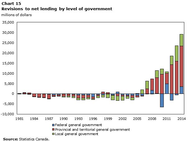
Description for Chart 15
The title of the graph is "Chart 15 Revisions to net lending by level of government."
This is a column stacked chart.
There are in total 34 categories in the horizontal axis. The vertical axis starts at -10,000 and ends at 35,000 with ticks every 5,000 points.
There are 3 series in this graph.
The vertical axis is "millions of dollars."
The units of the horizontal axis are years from 1981 to 2014.
The title of series 1 is "Federal general government."
The minimum value is -6,513 occurring in 2010.
The maximum value is 4,824 occurring in 2011.
The title of series 2 is "Provincial and territorial general government."
The minimum value is -2,078 occurring in 1987.
The maximum value is 19,778 occurring in 2014.
The title of series 3 is "Local general government."
The minimum value is -2,171 occurring in 2001.
The maximum value is 7,509 occurring in 2013.
| Federal general government | Provincial and territoiral general government | Local general government | |
|---|---|---|---|
| 1981 | 23 | -66 | 35 |
| 1982 | -92 | 429 | 28 |
| 1983 | -114 | 459 | -3 |
| 1984 | -56 | -1,338 | -47 |
| 1985 | -9 | -1,723 | -75 |
| 1986 | -159 | -1,659 | -98 |
| 1987 | -359 | -2,078 | -137 |
| 1988 | -580 | -683 | -135 |
| 1989 | -504 | -590 | -139 |
| 1990 | -228 | -976 | -392 |
| 1991 | -172 | -875 | -631 |
| 1992 | -265 | -999 | -767 |
| 1993 | -616 | -1,510 | -900 |
| 1994 | -601 | -1,569 | -844 |
| 1995 | -580 | -1,263 | -809 |
| 1996 | -1,452 | -1,004 | -473 |
| 1997 | -416 | -630 | -867 |
| 1998 | -537 | 931 | -1,107 |
| 1999 | -89 | 645 | -1,817 |
| 2000 | -535 | -298 | -2,153 |
| 2001 | 869 | -1,127 | -2,171 |
| 2002 | -660 | -578 | -1,883 |
| 2003 | -790 | -451 | -1,056 |
| 2004 | -825 | -1,038 | -1,190 |
| 2005 | -944 | -740 | 218 |
| 2006 | -951 | -283 | 1,968 |
| 2007 | -153 | 2,436 | 3,799 |
| 2008 | 1,594 | 5,702 | -42 |
| 2009 | 80 | 7,828 | 3,491 |
| 2010 | -6,513 | 9,486 | 2,691 |
| 2011 | 4,824 | 5,235 | 753 |
| 2012 | -3,141 | 14,194 | 4,371 |
| 2013 | -564 | 15,970 | 7,509 |
| 2014 | 3,564 | 19,778 | 5,860 |
| Source: Statistics Canada. | |||
7. Revisions to financial flows and balance sheets
Revisions to national wealth were substantial over the entire revision period. Canada’s national wealth represents the current market value of all non-financial assets (machinery, buildings, roads, bridges, factories, etc.) owned by residents of Canada. Revisions are the result of three factors. The first is a revision in the service lives attributed to non-financial assets. A recent study indicated that services lives previously used to depreciate Canada’s non-residential buildings were too high and they were therefore revised downwards. The result is a faster depreciation of the capital stock of non-residential buildings and a downward revision the fixed capital component of national wealth.
The second reason for the revision to national wealth is the addition of selected natural resources to Canada’s quarterly balance sheet, which had only been recorded in the consolidated annual balance sheet. Previously, resources such as exploitable oil reserves, timber resources, and mineral deposits were not included in Canada’s official measure of national wealth. These important assets have now been added to the national balance sheet as non-produced assets, reflecting their significant role in the production process. They are a key input into Canada’s economic growth and a significant factor in understanding the valuation of the non-financial portion of the balance sheet.
The third revision is due to improved estimates of the value of residential real estate held by households. Previously, the value of residential real estate (houses and land) was estimated using the perpetual inventory method for the value of housing, and a land-to-structure ratio to derive estimates of land. The latter methodology has been improved. Statistics Canada recently obtained access to municipal assessment files, which provide a much more current and accurate value of residential real estate. In addition, estimates from the most recent Survey of Financial Security indicated that an upward revision to land was required in order to properly estimate the value of residential real estate. Both the Survey of Financial Security and property assessment data are more reflective of the range of Canada’s residential real estate. These new data sources have been incorporated into the land estimate included in Canada’s national wealth.
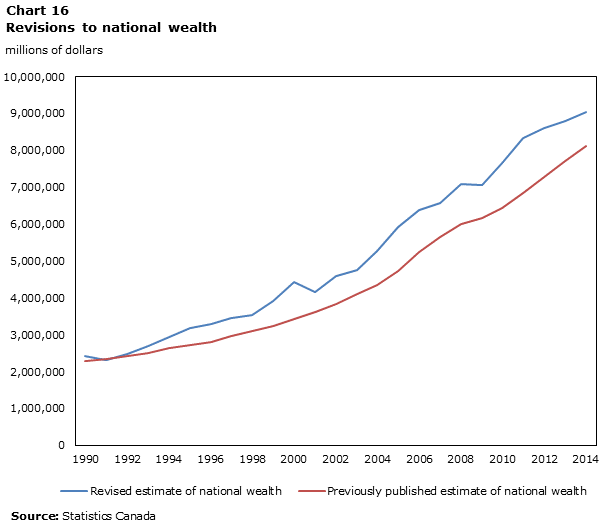
Description for Chart 16
The title of the graph is "Chart 16 Revisions to national wealth."
This is a line chart.
There are in total 25 categories in the horizontal axis. The vertical axis starts at 0 and ends at 10,000,000 with ticks every 1,000,000 points.
There are 2 series in this graph.
The vertical axis is "millions of dollars."
The units of the horizontal axis are years from 1990 to 2014.
The title of series 1 is "Revised estimate of national wealth."
The minimum value is 2,325,475 occurring in 1991.
The maximum value is 9,036,126 occurring in 2014.
The title of series 2 is "Previously published estimate of national wealth."
The minimum value is 2,292,004 occurring in 1990.
The maximum value is 8,127,427 occurring in 2014.
| Year | Revised estimate of national wealth | Previously published estimate of national wealth |
|---|---|---|
| 1990 | 2,419,116 | 2,292,004 |
| 1991 | 2,325,475 | 2,337,136 |
| 1992 | 2,484,450 | 2,412,416 |
| 1993 | 2,693,700 | 2,511,107 |
| 1994 | 2,937,422 | 2,633,558 |
| 1995 | 3,183,270 | 2,716,591 |
| 1996 | 3,294,875 | 2,813,569 |
| 1997 | 3,444,892 | 2,953,849 |
| 1998 | 3,543,700 | 3,090,300 |
| 1999 | 3,911,841 | 3,242,689 |
| 2000 | 4,418,498 | 3,420,513 |
| 2001 | 4,167,813 | 3,603,842 |
| 2002 | 4,591,065 | 3,824,395 |
| 2003 | 4,761,169 | 4,102,578 |
| 2004 | 5,271,022 | 4,348,404 |
| 2005 | 5,920,598 | 4,716,009 |
| 2006 | 6,370,100 | 5,235,027 |
| 2007 | 6,564,081 | 5,657,135 |
| 2008 | 7,094,572 | 5,992,968 |
| 2009 | 7,071,982 | 6,177,956 |
| 2010 | 7,661,456 | 6,445,949 |
| 2011 | 8,330,638 | 6,845,495 |
| 2012 | 8,598,962 | 7,271,697 |
| 2013 | 8,793,297 | 7,707,683 |
| 2014 | 9,036,126 | 8,127,427 |
| Source: Statistics Canada | ||
Household credit market debt
There was little revision to household credit market debt over the revision period. The revised estimates continue to show a steady increase in the level of household mortgage and other credit market debt.
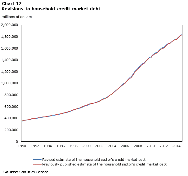
Description for Chart 17
The title of the graph is "Chart 17 Revisions to household credit market debt."
This is a line chart.
There are in total 100 categories in the horizontal axis. The vertical axis starts at 0 and ends at 2,000,000 with ticks every 200,000 points.
There are 2 series in this graph.
The vertical axis is "millions of dollars."
The units of the horizontal axis are quarters by year from first quarter 1990 to fourth quarter 2014.
The title of series 1 is "Revised estimate of the household sector's credit market debt."
The minimum value is 348,869 occurring in first quarter 1990.
The maximum value is 1,832,199 occurring in fourth quarter 2014.
The title of series 2 is "Previously published estimate of the household sector's credit market debt."
The minimum value is 352,746 occurring in first quarter 1990.
The maximum value is 1,828,421 occurring in fourth quarter 2014.
| Revised estimate of the household sector's credit market debt |
Previously published estimate of the household sector's credit market debt |
|
|---|---|---|
| 1990Q1 | 348,869 | 352,746 |
| 1990Q2 | 358,314 | 363,225 |
| 1990Q3 | 362,667 | 366,502 |
| 1990Q4 | 367,353 | 371,857 |
| 1991Q1 | 368,880 | 373,634 |
| 1991Q2 | 375,926 | 378,649 |
| 1991Q3 | 383,313 | 389,090 |
| 1991Q4 | 386,683 | 392,404 |
| 1992Q1 | 389,227 | 395,375 |
| 1992Q2 | 395,554 | 401,937 |
| 1992Q3 | 400,423 | 409,534 |
| 1992Q4 | 407,837 | 418,868 |
| 1993Q1 | 407,833 | 415,933 |
| 1993Q2 | 416,458 | 424,000 |
| 1993Q3 | 420,761 | 424,347 |
| 1993Q4 | 425,169 | 428,651 |
| 1994Q1 | 428,089 | 432,588 |
| 1994Q2 | 433,729 | 437,734 |
| 1994Q3 | 439,920 | 444,409 |
| 1994Q4 | 449,065 | 452,548 |
| 1995Q1 | 450,060 | 455,456 |
| 1995Q2 | 453,820 | 458,367 |
| 1995Q3 | 463,002 | 467,783 |
| 1995Q4 | 467,066 | 470,257 |
| 1996Q1 | 471,052 | 477,696 |
| 1996Q2 | 478,735 | 484,004 |
| 1996Q3 | 484,785 | 490,884 |
| 1996Q4 | 491,711 | 499,380 |
| 1997Q1 | 498,863 | 504,947 |
| 1997Q2 | 505,657 | 511,691 |
| 1997Q3 | 520,258 | 523,809 |
| 1997Q4 | 529,544 | 536,346 |
| 1998Q1 | 538,773 | 545,409 |
| 1998Q2 | 546,633 | 551,990 |
| 1998Q3 | 558,505 | 563,617 |
| 1998Q4 | 567,641 | 571,326 |
| 1999Q1 | 573,709 | 579,356 |
| 1999Q2 | 584,687 | 591,951 |
| 1999Q3 | 595,648 | 603,704 |
| 1999Q4 | 606,374 | 614,767 |
| 2000Q1 | 616,001 | 621,570 |
| 2000Q2 | 626,170 | 633,121 |
| 2000Q3 | 638,725 | 644,288 |
| 2000Q4 | 646,684 | 652,048 |
| 2001Q1 | 649,095 | 652,921 |
| 2001Q2 | 660,388 | 662,958 |
| 2001Q3 | 672,910 | 669,432 |
| 2001Q4 | 683,292 | 678,594 |
| 2002Q1 | 693,310 | 689,695 |
| 2002Q2 | 711,282 | 705,932 |
| 2002Q3 | 727,526 | 718,261 |
| 2002Q4 | 740,497 | 732,599 |
| 2003Q1 | 746,641 | 742,726 |
| 2003Q2 | 762,878 | 758,248 |
| 2003Q3 | 784,495 | 780,701 |
| 2003Q4 | 803,008 | 799,641 |
| 2004Q1 | 814,571 | 813,029 |
| 2004Q2 | 846,468 | 844,226 |
| 2004Q3 | 869,572 | 865,993 |
| 2004Q4 | 892,472 | 888,476 |
| 2005Q1 | 913,050 | 905,955 |
| 2005Q2 | 940,523 | 930,786 |
| 2005Q3 | 967,909 | 958,079 |
| 2005Q4 | 989,929 | 983,289 |
| 2006Q1 | 1,008,672 | 999,762 |
| 2006Q2 | 1,036,505 | 1,026,368 |
| 2006Q3 | 1,066,918 | 1,054,349 |
| 2006Q4 | 1,096,542 | 1,082,291 |
| 2007Q1 | 1,118,596 | 1,102,224 |
| 2007Q2 | 1,158,848 | 1,142,283 |
| 2007Q3 | 1,197,508 | 1,181,824 |
| 2007Q4 | 1,225,933 | 1,211,956 |
| 2008Q1 | 1,251,767 | 1,238,632 |
| 2008Q2 | 1,289,463 | 1,276,137 |
| 2008Q3 | 1,321,100 | 1,305,630 |
| 2008Q4 | 1,339,228 | 1,324,617 |
| 2009Q1 | 1,347,398 | 1,342,583 |
| 2009Q2 | 1,379,268 | 1,376,223 |
| 2009Q3 | 1,408,900 | 1,404,987 |
| 2009Q4 | 1,437,786 | 1,432,764 |
| 2010Q1 | 1,448,980 | 1,435,251 |
| 2010Q2 | 1,479,608 | 1,467,999 |
| 2010Q3 | 1,502,365 | 1,490,010 |
| 2010Q4 | 1,523,478 | 1,512,714 |
| 2011Q1 | 1,530,441 | 1,518,702 |
| 2011Q2 | 1,562,665 | 1,550,193 |
| 2011Q3 | 1,587,883 | 1,575,774 |
| 2011Q4 | 1,608,410 | 1,594,202 |
| 2012Q1 | 1,614,329 | 1,602,943 |
| 2012Q2 | 1,640,007 | 1,629,098 |
| 2012Q3 | 1,665,611 | 1,657,978 |
| 2012Q4 | 1,681,199 | 1,676,354 |
| 2013Q1 | 1,686,066 | 1,683,501 |
| 2013Q2 | 1,712,155 | 1,709,521 |
| 2013Q3 | 1,737,551 | 1,733,020 |
| 2013Q4 | 1,751,696 | 1,745,691 |
| 2014Q1 | 1,756,895 | 1,753,480 |
| 2014Q2 | 1,784,886 | 1,780,241 |
| 2014Q3 | 1,812,193 | 1,807,804 |
| 2014Q4 | 1,832,199 | 1,828,421 |
| Source: Statistics Canada | ||
The revision to the ratio of household credit market debt to disposable income was minimal over the period due to the correspondingly small revisions to the level of household credit market debt. Additionally, disposable income used in the calculation of this ratio excludes transactions relating to pension funds. This was done to maintain international comparability and time series consistency with our major partners.
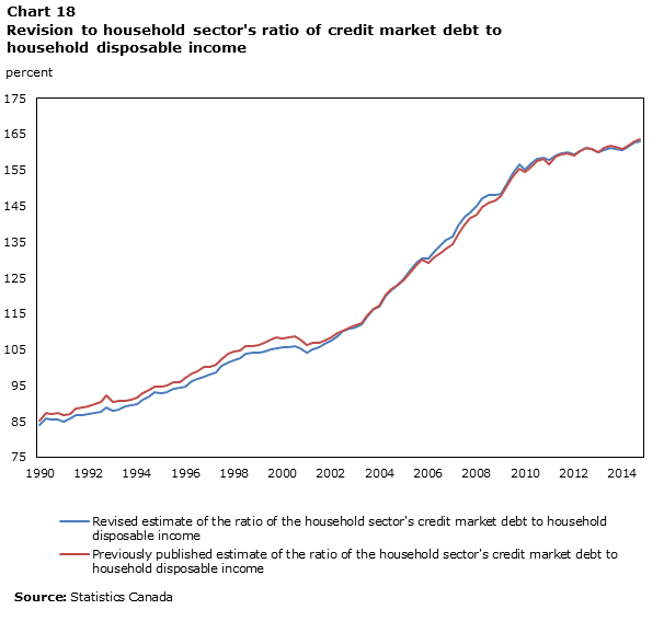
Description for Chart 18
The title of the graph is "Chart 18 Revisions to household credit market debt."
This is a line chart.
There are in total 100 categories in the horizontal axis. The vertical axis starts at 75 and ends at 175 with ticks every 10 points.
There are 2 series in this graph.
The vertical axis is "percent."
The units of the horizontal axis are quarters by year from first quarter 1990 to fourth quarter 2014.
The title of series 1 is "Revised estimate of the ratio of the household sector's credit market debt to household disposable income."
The minimum value is 84.1 occurring in first quarter 1990.
The maximum value is 163 occurring in fourth quarter 2014.
The title of series 2 is "Previously published estimate of the ratio of the household sector's credit market debt to household disposable income."
The minimum value is 85.3 occurring in first quarter 1990.
The maximum value is 163.6 occurring in fourth quarter 2014.
| Revised estimate of the ratio of the household sector's credit market debt to household disposable income |
Previously published estimate of the ratio of the household sector's credit market debt to household disposable income |
|
|---|---|---|
| 1990Q1 | 84.1 | 85.3 |
| 1990Q2 | 85.8 | 87.4 |
| 1990Q3 | 85.6 | 87.1 |
| 1990Q4 | 85.5 | 87.2 |
| 1991Q1 | 85.0 | 86.8 |
| 1991Q2 | 85.7 | 86.9 |
| 1991Q3 | 86.6 | 88.6 |
| 1991Q4 | 86.8 | 88.8 |
| 1992Q1 | 87.0 | 89.1 |
| 1992Q2 | 87.5 | 89.7 |
| 1992Q3 | 87.6 | 90.5 |
| 1992Q4 | 88.9 | 92.1 |
| 1993Q1 | 88.0 | 90.5 |
| 1993Q2 | 88.3 | 90.6 |
| 1993Q3 | 89.1 | 90.6 |
| 1993Q4 | 89.6 | 91.1 |
| 1994Q1 | 89.8 | 91.5 |
| 1994Q2 | 91.1 | 92.8 |
| 1994Q3 | 92.0 | 93.8 |
| 1994Q4 | 93.1 | 94.8 |
| 1995Q1 | 92.7 | 94.8 |
| 1995Q2 | 93.0 | 94.9 |
| 1995Q3 | 94.1 | 96.0 |
| 1995Q4 | 94.3 | 95.9 |
| 1996Q1 | 94.7 | 97.0 |
| 1996Q2 | 96.2 | 98.2 |
| 1996Q3 | 96.8 | 99.0 |
| 1996Q4 | 97.5 | 100.1 |
| 1997Q1 | 98.0 | 100.3 |
| 1997Q2 | 98.5 | 100.8 |
| 1997Q3 | 100.5 | 102.3 |
| 1997Q4 | 101.3 | 103.7 |
| 1998Q1 | 101.9 | 104.3 |
| 1998Q2 | 102.5 | 104.7 |
| 1998Q3 | 103.7 | 105.9 |
| 1998Q4 | 104.0 | 105.9 |
| 1999Q1 | 104.0 | 106.3 |
| 1999Q2 | 104.5 | 107.0 |
| 1999Q3 | 105.1 | 107.8 |
| 1999Q4 | 105.5 | 108.4 |
| 2000Q1 | 105.6 | 108.1 |
| 2000Q2 | 105.7 | 108.5 |
| 2000Q3 | 106.0 | 108.6 |
| 2000Q4 | 105.3 | 107.8 |
| 2001Q1 | 104.0 | 106.2 |
| 2001Q2 | 104.9 | 106.9 |
| 2001Q3 | 105.8 | 106.9 |
| 2001Q4 | 106.6 | 107.5 |
| 2002Q1 | 107.4 | 108.4 |
| 2002Q2 | 108.8 | 109.5 |
| 2002Q3 | 110.1 | 110.2 |
| 2002Q4 | 110.9 | 111.1 |
| 2003Q1 | 111.0 | 111.7 |
| 2003Q2 | 112.0 | 112.4 |
| 2003Q3 | 114.2 | 114.5 |
| 2003Q4 | 116.2 | 116.4 |
| 2004Q1 | 116.9 | 117.3 |
| 2004Q2 | 120.1 | 120.3 |
| 2004Q3 | 121.6 | 121.8 |
| 2004Q4 | 123.0 | 123.0 |
| 2005Q1 | 124.5 | 124.2 |
| 2005Q2 | 127.1 | 126.4 |
| 2005Q3 | 129.2 | 128.4 |
| 2005Q4 | 130.5 | 130.1 |
| 2006Q1 | 130.4 | 129.2 |
| 2006Q2 | 132.2 | 130.6 |
| 2006Q3 | 134.0 | 132.0 |
| 2006Q4 | 135.4 | 133.0 |
| 2007Q1 | 136.6 | 134.3 |
| 2007Q2 | 139.6 | 137.2 |
| 2007Q3 | 142.0 | 139.9 |
| 2007Q4 | 143.3 | 141.5 |
| 2008Q1 | 145.1 | 142.5 |
| 2008Q2 | 147.2 | 144.7 |
| 2008Q3 | 148.0 | 145.8 |
| 2008Q4 | 148.2 | 146.5 |
| 2009Q1 | 148.4 | 147.8 |
| 2009Q2 | 151.4 | 150.7 |
| 2009Q3 | 154.3 | 153.2 |
| 2009Q4 | 156.5 | 155.4 |
| 2010Q1 | 155.2 | 154.6 |
| 2010Q2 | 156.9 | 156.1 |
| 2010Q3 | 158.0 | 157.5 |
| 2010Q4 | 158.3 | 158.2 |
| 2011Q1 | 157.7 | 156.6 |
| 2011Q2 | 159.1 | 158.7 |
| 2011Q3 | 159.7 | 159.3 |
| 2011Q4 | 160.1 | 159.5 |
| 2012Q1 | 159.2 | 159.0 |
| 2012Q2 | 160.4 | 160.2 |
| 2012Q3 | 161.1 | 161.1 |
| 2012Q4 | 161.0 | 161.0 |
| 2013Q1 | 159.8 | 160.0 |
| 2013Q2 | 160.6 | 161.1 |
| 2013Q3 | 161.2 | 161.7 |
| 2013Q4 | 160.9 | 161.5 |
| 2014Q1 | 160.6 | 160.8 |
| 2014Q2 | 161.6 | 161.7 |
| 2014Q3 | 162.8 | 163.0 |
| 2014Q4 | 163.0 | 163.6 |
| Source: Statistics Canada | ||
Currency and deposits – non-financial corporations
Statistics Canada uses aggregate information, provided by Canadian chartered banks and other deposit-taking institutions, to estimate the stock of currency and deposits by sector. This information is supplied by type of deposit (for example, demand and notice, and fixed term deposit) and depositor sector. Additionally, this information follows prevailing business accounting rules in classifying chartered bank deposit liabilities. As such, they include covered bonds, bearer-deposit notes, and other securities issued by chartered banks in order to obtain funding. To better align with recommended international macroeconomic accounting standards, these bank liabilities have been re-classified to bonds and other short-term securities from currency and deposits. This re-classification strengthens the estimates, and will better depict the flow of funds by instrument in the economy. As a result of this change in classification, financial corporations (for example, pension funds and insurance companies) bonds and short-term securities were revised, as well as, the currency and deposits held by private non-financial corporations (shown in Chart 19). With this improved classification of instruments within the NBSA, the data still show a strong upward trend in both the overall liquidity and value of currency and deposits held by non-financial private corporations.
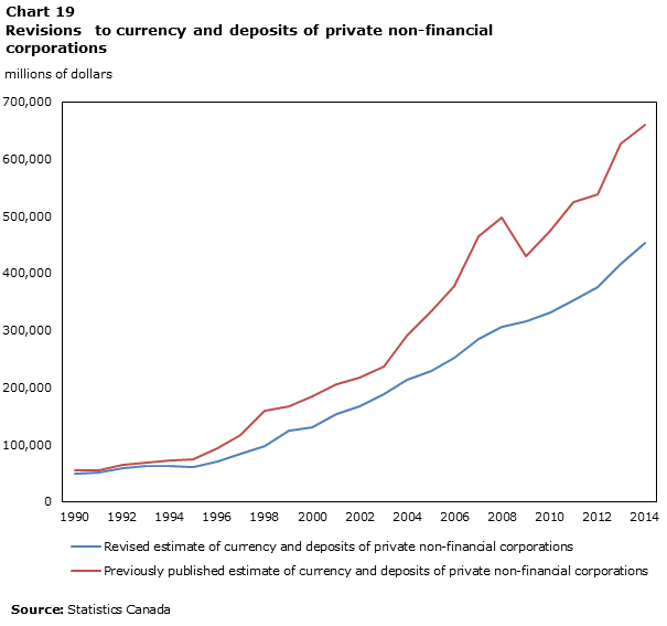
Description for Chart 19
The title of the graph is "Chart 19 Revisions to currency and deposits of private non-financial corporations."
This is a line chart.
There are in total 25 categories in the horizontal axis. The vertical axis starts at 0 and ends at 700,000 with ticks every 100,000 points.
There are 2 series in this graph.
The vertical axis is "millions of dollars."
The units of the horizontal axis are years from 1990 to 2014.
The title of series 1 is "Current estimate of currency and deposits of private non-financial corporations."
The minimum value is 49,063 occurring in 1990.
The maximum value is 453,868 occurring in 2014.
The title of series 2 is "Previously published estimate of currency and deposits of private non-financial corporations."
The minimum value is 54,619 occurring in 1991.
The maximum value is 659,420 occurring in 2014.
| Year | Current estimate of currency and deposits of private non-financial corporations |
Previously published estimate of currency and deposits of private non-financial corporations |
|---|---|---|
| 1990 | 49,063 | 54,843 |
| 1991 | 51,230 | 54,619 |
| 1992 | 58,166 | 63,821 |
| 1993 | 61,643 | 68,926 |
| 1994 | 62,244 | 71,535 |
| 1995 | 59,612 | 74,517 |
| 1996 | 69,704 | 93,954 |
| 1997 | 83,549 | 116,374 |
| 1998 | 97,198 | 159,620 |
| 1999 | 123,853 | 167,172 |
| 2000 | 130,516 | 183,574 |
| 2001 | 153,789 | 205,428 |
| 2002 | 166,191 | 216,799 |
| 2003 | 187,704 | 236,996 |
| 2004 | 214,029 | 290,025 |
| 2005 | 229,371 | 332,555 |
| 2006 | 251,482 | 377,619 |
| 2007 | 284,367 | 463,889 |
| 2008 | 305,678 | 498,538 |
| 2009 | 315,030 | 430,010 |
| 2010 | 331,410 | 474,817 |
| 2011 | 352,102 | 525,267 |
| 2012 | 375,736 | 539,064 |
| 2013 | 416,512 | 626,603 |
| 2014 | 453,868 | 659,420 |
| Source: Statistics Canada | ||
General government debt
There was a downward revision to general governments’ debt over the time period of the revision. The majority of the revision occurred in the 2006 to 2014 period, resulting primarily from the incorporation of the new government finance statistics into the macroeconomic accounts framework. Debt levels were revised downward for all levels of government (federal, provincial and territorial, local and Aboriginal general governments), although the revisions to the federal level were less substantial.
| Time period | Revised average estimate of federal general government credit market debt | Previously published average estimate of general government credit market debt | Revision to the estimate of federal general government credit market debt | Current average estimate of other general government credit market debt | Previously published average estimate of other general government credit market debt | Revision to the estimate of other general government credit market debt |
|---|---|---|---|---|---|---|
| millions of dollars | ||||||
| 1990 to 1999 | 416,772 | 416,780 | -8 | 277,867 | 273,223 | 4,644 |
| 2000 to 2009 | 436,615 | 435,031 | 1,584 | 425,216 | 407,663 | 17,554 |
| 2010 to 2014 | 643,783 | 630,421 | 13,362 | 695,828 | 650,488 | 45,340 |
| Entire period | 470,111 | 466,809 | 3,303 | 420,399 | 402,452 | 17,947 |
| Source: Statistics Canada | ||||||
The downward revision in debt levels resulted in an upward revision in the ratio of general government net debt to gross domestic product.
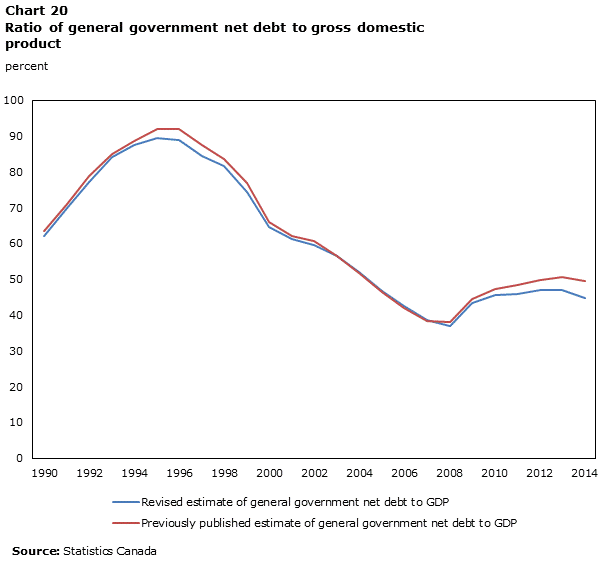
Description for Chart 20
The title of the graph is "Chart 20 Ratio of federal government net debt to gross domestic product."
This is a line chart.
There are in total 25 categories in the horizontal axis. The vertical axis starts at 0 and ends at 100 with ticks every 10 points.
There are 2 series in this graph.
The vertical axis is "percent."
The units of the horizontal axis are years from 1990 to 2014.
The title of series 1 is "Revised estimate of general government net debt to GDP."
The minimum value is 36.9 occurring in 2008.
The maximum value is 89.4 occurring in 1995.
The title of series 2 is "Previously published estimate of general government net debt to GDP."
The minimum value is 38 occurring in 2008.
The maximum value is 92.1 occurring in 1996.
| Year | Revised estimate of general government net debt to GDP |
Previously published estimate of general government net debt to GDP |
|---|---|---|
| 1990 | 62.0 | 63.4 |
| 1991 | 70.0 | 70.9 |
| 1992 | 77.3 | 78.8 |
| 1993 | 84.1 | 85.0 |
| 1994 | 87.6 | 88.7 |
| 1995 | 89.4 | 92.0 |
| 1996 | 88.8 | 92.1 |
| 1997 | 84.3 | 87.4 |
| 1998 | 81.7 | 83.5 |
| 1999 | 74.3 | 76.8 |
| 2000 | 64.6 | 66.0 |
| 2001 | 61.2 | 62.1 |
| 2002 | 59.7 | 60.8 |
| 2003 | 56.5 | 56.6 |
| 2004 | 51.9 | 51.8 |
| 2005 | 46.7 | 46.4 |
| 2006 | 42.4 | 42.1 |
| 2007 | 38.6 | 38.3 |
| 2008 | 36.9 | 38.0 |
| 2009 | 43.5 | 44.6 |
| 2010 | 45.7 | 47.2 |
| 2011 | 45.9 | 48.3 |
| 2012 | 46.9 | 49.9 |
| 2013 | 46.9 | 50.5 |
| 2014 | 44.7 | 49.4 |
| Source: Statistics Canada | ||
Pension assets and liabilities
Pension assets were also revised as a result of the new accrual-based treatment of pensions. In the past, pension assets were recorded on a cash basis—meaning that the asset was only recognized when a cash payment was made to the fund by the contributors. Depending on the actuarial outlook of a fund, employers often took contribution holidays, which were sometimes followed by large lump-sum ‘catch-up’ payments. This resulted in a somewhat volatile profile of the asset through time. In that scenario, it was not possible to have a true picture of pension assets owing to the household sector at any point in time. The move to record pension contributions on an entitlement basis resulted in a revision to the profile of pension assets and liabilities in the financial corporations’ sector and the household sector, providing a more accurate picture of their true assets and liabilities.
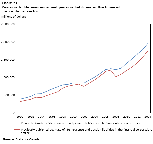
Description for Chart 21
The title of the graph is "Chart 21 Revision to life insurance and pension liabilities in the financial corporations sector."
This is a line chart.
There are in total 25 categories in the horizontal axis. The vertical axis starts at 0 and ends at 2,500,000 with ticks every 500,000 points.
There are 2 series in this graph.
The vertical axis is "millions of dollars."
The units of the horizontal axis are years from 1990 to 2014.
The title of series 1 is "Revised estimate of life insurance and pension liabilities in the financial corporations sector."
The minimum value is 386,025 occurring in 1990.
The maximum value is 1,962,528 occurring in 2014.
The title of series 2 is "Previously published estimate of life insurance and pension liabilities in the financial corporations sector."
The minimum value is 315,325 occurring in 1990.
The maximum value is 1,745,832 occurring in 2014.
| Time period | Revised estimate of life insurance and pension liabilities in the financial corporations sector |
Previously published estimate of life insurance and pension liabilities in the financial corporations sector |
|---|---|---|
| 1990 | 386,025 | 315,325 |
| 1991 | 423,428 | 353,164 |
| 1992 | 466,706 | 380,177 |
| 1993 | 540,096 | 446,423 |
| 1994 | 544,043 | 429,486 |
| 1995 | 612,331 | 485,973 |
| 1996 | 676,624 | 548,706 |
| 1997 | 733,568 | 597,244 |
| 1998 | 789,752 | 697,124 |
| 1999 | 801,110 | 751,875 |
| 2000 | 846,266 | 784,116 |
| 2001 | 836,187 | 810,146 |
| 2002 | 840,355 | 748,800 |
| 2003 | 924,036 | 840,143 |
| 2004 | 1,010,047 | 933,277 |
| 2005 | 1,110,900 | 1,040,659 |
| 2006 | 1,215,756 | 1,170,281 |
| 2007 | 1,246,691 | 1,206,021 |
| 2008 | 1,215,882 | 1,026,728 |
| 2009 | 1,262,178 | 1,095,354 |
| 2010 | 1,395,833 | 1,190,737 |
| 2011 | 1,527,809 | 1,287,115 |
| 2012 | 1,654,645 | 1,408,130 |
| 2013 | 1,781,315 | 1,573,553 |
| 2014 | 1,962,528 | 1,745,832 |
| Source: Statistics Canada | ||
Other changes in assets account
The Canadian System of National Accounts is an integrated sequence of accounts. It consists of production accounts and a host of sector accounts including: income and outlay accounts, capital and finance accounts (financial flow accounts), and the national balance sheet accounts. However, one element of the sequence, the other changes in assets account—comprised of other changes in the volume of assets account and the revaluation account—although available implicitly, is not published. This component account constitutes the missing link between the flows recorded in the transactions' accounts and stocks recorded in the balance sheet.
Although it might be assumed that the flow of financial assets into a sector each year would represent the change in the sector’s stock of financial assets, this is not the case, as seen in Chart 22 for the domestic economy. In fact, the ‘other changes’ (led by revaluations) far outweigh the financial flows. This other changes represent the change in financial assets due to changes in the price (largely fluctuations in the price of equities held directly or indirectly by the household sector).
The revaluation account represents the change in the monetary value of an asset or liability due to changes in the level and structure of its price. These revaluations are generally separated led by two sub-components: exchange rate changes and market price changes.
The other changes in the volume of assets account represents changes in the value of assets that are neither due to transactions nor revaluation. Examples include write-ups/downs of assets, economic appearance and disappearance of assets, reclassifications and changes in financial assets resulting from institutional units changing institutional sectors.
Description for Chart 22
The title of the graph is "Chart 22 Total Financial assets of domestic economy."
This is a column stacked chart.
There are in total 31 categories in the horizontal axis. The vertical axis starts at -1,000,000 and ends at 800,000 with ticks every 200,000 points.
There are 2 series in this graph.
The vertical axis is "millions of dollars."
The units of the horizontal axis are quarters by year from second quarter 2007 to fourth quarter 2014.
The title of series 1 is "Financial flows."
The minimum value is 25,626 occurring in fourth quarter 2010.
The maximum value is 421,880 occurring in fourth quarter 2008.
The title of series 2 is "Other change in assets."
The minimum value is -817,001 occurring in third quarter 2008.
The maximum value is 489,346 occurring in fourth quarter 2013.
| Quarter | Financial flows | Other change in assets |
|---|---|---|
| 2007Q2 | 224,194 | 128,659 |
| 2007Q3 | 196,266 | 74,285 |
| 2007Q4 | 159,071 | - 148,942 |
| 2008Q1 | 319,042 | 23,813 |
| 2008Q2 | 161,969 | - 86,310 |
| 2008Q3 | 155,207 | - 817,001 |
| 2008Q4 | 421,880 | - 510,162 |
| 2009Q1 | 72,477 | - 62,469 |
| 2009Q2 | 28,549 | 439,105 |
| 2009Q3 | 123,288 | 427,484 |
| 2009Q4 | 153,155 | 115,634 |
| 2010Q1 | 237,448 | - 2,264 |
| 2010Q2 | 147,760 | - 97,342 |
| 2010Q3 | 236,465 | 429,401 |
| 2010Q4 | 25,626 | 371,534 |
| 2011Q1 | 261,295 | 273,650 |
| 2011Q2 | 173,628 | - 106,587 |
| 2011Q3 | 227,185 | - 348,667 |
| 2011Q4 | 64,890 | 55,941 |
| 2012Q1 | 117,646 | 488,581 |
| 2012Q2 | 107,045 | - 168,590 |
| 2012Q3 | 163,517 | 225,760 |
| 2012Q4 | 105,540 | 107,512 |
| 2013Q1 | 244,808 | 409,710 |
| 2013Q2 | 176,839 | - 151,615 |
| 2013Q3 | 117,507 | 192,138 |
| 2013Q4 | 42,493 | 489,346 |
| 2014Q1 | 81,536 | 268,424 |
| 2014Q2 | 141,385 | 137,839 |
| 2014Q3 | 215,241 | 35,869 |
| 2014Q4 | 147,680 | 352,999 |
| Source: Statistics Canada. | ||
The international standard recommends that the other changes in assets account be broken into its component accounts: revaluation account and other changes in the volume of assets account. Statistics Canada is currently unable to provide this detail, but will release the aggregate other changes in assets account. The goal of this account is to provide data users with insight into how wealth is generated in each of the sectors of the economy. Changes in wealth—increases or decreases—due to saving are articulated in the financial account, while changes in wealth due to a price or volume change are articulated in the other changes in assets account.
8. Revisions to gross domestic product by province and territory
Given that the sizes of the provincial and territorial economies differ significantly, revisions across the provinces and territories are examined in terms of their relative size. The average revised level of gross domestic product is compared to the previously published average level of gross domestic product for the period 1981 to 2013.
The largest downward revisions occurred in Nunavut and Newfoundland and Labrador while the largest upward revision occurred in Manitoba and New Brunswick. The smallest revisions occurred in Prince Edward Island, Saskatchewan and Quebec.
| Province/Territory | Revised estimate of the average level of gross domestic product (1981 to 2013) | Previously published estimate of the average level of gross domestic product (1981 to 2013) | Revised estimate of the average level of gross domestic product (1981 to 2013) as a share of the previously published estimate |
|---|---|---|---|
| millions of dollars | percent | ||
| Newfoundland and Labrador | 15,559 | 15,672 | 99.28 |
| Prince Edward Island | 3,135 | 3,138 | 99.90 |
| Nova Scotia | 23,488 | 23,595 | 99.55 |
| New Brunswick | 19,032 | 18,918 | 100.60 |
| Quebec | 210,674 | 211,017 | 99.84 |
| Ontario | 400,241 | 398,413 | 100.46 |
| Manitoba | 33,497 | 33,253 | 100.73 |
| Saskatchewan | 35,437 | 35,480 | 99.88 |
| Alberta | 145,990 | 145,241 | 100.52 |
| British Columbia | 124,399 | 124,149 | 100.20 |
| Yukon | 1,304 | 1,300 | 100.31 |
| Northwest TerritoriesNote 1 | 4,058 | 4,043 | 100.37 |
| NunavutNote 1 | 1,407 | 1,429 | 98.46 |
|
|||
Revisions to growth in real gross domestic product by province and territory were minimal over the revision period. The average absolute mean revision to real gross domestic product ranged between a high of 1.47 percentage points in Nunavut to a low of 0.15 percentage points in Ontario. In terms of average growth over the 1981 to 2013 period, Alberta remains the province with the largest growth rate, averaging a 3.13% annual real growth over the period followed by Ontario then Newfoundland and Labrador. Nunavut remained the fastest growing territory.
| Province or territory | Revised estimate of the average growth in real gross domestic product (1982 to 2013) | Previously published estimate of the average growth in real gross domestic product (1982 to 2013) | Average absolute revision to real gross domestic product |
|---|---|---|---|
| percent | |||
| Newfoundland and Labrador | 2.59 | 2.64 | 0.32 |
| Prince Edward Island | 2.47 | 2.50 | 0.56 |
| Nova Scotia | 1.95 | 1.95 | 0.25 |
| New Brunswick | 2.03 | 2.01 | 0.23 |
| Quebec | 1.93 | 1.95 | 0.19 |
| Ontario | 2.59 | 2.62 | 0.15 |
| Manitoba | 2.11 | 2.10 | 0.17 |
| Saskatchewan | 2.18 | 2.28 | 0.30 |
| Alberta | 3.13 | 3.14 | 0.36 |
| British Columbia | 2.47 | 2.48 | 0.17 |
| Yukon | 3.75 | 3.69 | 0.64 |
| Northwest TerritoriesNote 1 Table 12 | 2.51 | 2.58 | 0.54 |
| NunavutNote 1 Table 12 | 4.92 | 4.68 | 1.47 |
|
|||
The relative size of the provincial economies did not change with this revision. Ontario remained the largest province, accounting for an average of 39.4% of the total national gross domestic product. This was followed by Quebec and then Alberta. The relative size of the provinces and territories remained unchanged in 2013, with Ontario accounting for the largest share of national gross domestic product followed by Quebec, with Alberta a close third.
| Province or territory | Revised average share of national gross domestic product (1981 to 2013) | Previously published average share of national gross domestic product (1981 to 2013) | Revised share of national gross domestic product (2013) | Previously published share of national gross domestic product (2013) |
|---|---|---|---|---|
| percent | ||||
| Newfoundland and Labrador | 1.5 | 1.5 | 1.8 | 1.9 |
| Prince Edward Island | 0.3 | 0.3 | 0.3 | 0.3 |
| Nova Scotia | 2.3 | 2.3 | 2.0 | 2.1 |
| New Brunswick | 1.9 | 1.9 | 1.7 | 1.7 |
| Quebec | 20.8 | 20.8 | 19.1 | 19.2 |
| Ontario | 39.4 | 39.2 | 36.6 | 36.8 |
| Manitoba | 3.3 | 3.3 | 3.3 | 3.2 |
| Saskatchewan | 3.5 | 3.5 | 4.4 | 4.4 |
| Alberta | 14.4 | 14.3 | 18.2 | 17.9 |
| British Columbia | 12.3 | 12.2 | 12.0 | 12.1 |
| Yukon | 0.1 | 0.1 | 0.1 | 0.1 |
| Northwest TerritoriesNote 1 Table 13 | 0.4 | 0.4 | 0.2 | 0.2 |
| NunavutNote 1 Table 13 | 0.1 | 0.1 | 0.1 | 0.1 |
|
||||
The majority of the revision to the provincial and territorial gross domestic product was due to the incorporation of revised estimates of government revenues and expenditures. The methodology, accounting and data sources used to compile the government revenues and expenditures by province and territory were improved significantly with this revision to the Provincial and Territorial Economic Accounts. Previous estimates of provincial general government revenues and expenditures were sourced from annual aggregate public account documents. With this revision, the estimates of government revenue and expenditures have been constructed from provincial government general ledger files. This improved data source permitted improved coding, coverage and classification of government revenues and expenditures, according to the latest international accounting standards.
| Province or territory | Average absolute revision to the level of general government final consumption expenditure (1981 to 2013) | Average absolute revision to the level of gross domestic product (1981 to 2013) | General government share of total revision |
|---|---|---|---|
| millions of dollars | percent | ||
| Newfoundland and Labrador | 140 | 140 | 1.00 |
| Prince Edward Island | 30 | 19 | 1.60 |
| Nova Scotia | 171 | 141 | 1.22 |
| New Brunswick | 138 | 133 | 1.04 |
| Quebec | 823 | 508 | 1.62 |
| Ontario | 1725 | 2017 | 0.86 |
| Manitoba | 117 | 244 | 0.48 |
| Saskatchewan | 238 | 132 | 1.80 |
| Alberta | 271 | 1015 | 0.27 |
| British Columbia | 389 | 609 | 0.64 |
| Yukon | 16 | 15 | 1.10 |
| Northwest TerritoriesNote 1 Table 14 | 29 | 29 | 1.00 |
| NunavutNote 1 Table 14 | 28 | 23 | 1.24 |
|
|||
In many cases the average absolute revision to general government final consumption expenditure is as large, or larger, than the average absolute revision to the level of gross domestic product for the provinces and territories. Revisions to general government final consumption expenditure were particularly large in Saskatchewan and Quebec. Revisions were more muted in Alberta and Manitoba.

Description for Chart 23
The title of the graph is "Chart 23 National share of general government final consumption expenditure by province and territory."
This is a column clustered chart.
There are in total 13 categories in the horizontal axis. The vertical axis starts at 0 and ends at 40 with ticks every 5 points.
There are 2 series in this graph.
The vertical axis is "provincial/territorial general government final consumption expenditure as a percent of the national total."
The horizontal axis is "province/territory."
The title of series 1 is "Revised average share of national general government final consumption expenditure (1981 to 2013)."
The minimum value is 0.3 and it corresponds to "Y.T.."
The maximum value is 36.9 and it corresponds to "Ont.."
The title of series 2 is "Previously published average share of national general government final consumption expenditure (1981 to 2013)."
The minimum value is 0.3 and it corresponds to "Y.T.."
The maximum value is 36.8 and it corresponds to "Ont.."
| Province or territory | Revised average share of national general government final consumption expenditure (1981 to 2013) | Previously published average share of national general government final consumption expenditure (1981 to 2013) |
|---|---|---|
| N.L. | 2.0 | 2.0 |
| P.E.I. | 0.5 | 0.5 |
| N.S. | 3.7 | 3.6 |
| N.B. | 2.6 | 2.6 |
| Que. | 23.2 | 23.4 |
| Ont. | 36.9 | 36.8 |
| Man. | 4.1 | 4.0 |
| Sask. | 3.4 | 3.5 |
| Alta. | 10.5 | 10.4 |
| B.C. | 11.6 | 11.6 |
| Y.T. | 0.3 | 0.3 |
| N.W.T. | 0.7 | 0.7 |
| Nvt. | 0.5 | 0.5 |
| Source: Statistics Canada | ||
Each province and territory’s share of total national general government final consumption expenditure was virtually unchanged with the 2015 comprehensive revision.
The revised treatment of defined benefit pension plans had an impact on the general government final consumption expenditure time series. Pension payments by governments are now recorded on an entitlement basis rather than on a cash basis. This served to smooth out the general government final consumption expenditure time series for a number of provinces. The following chart shows the previously published general government final consumption expenditure series and the revised series for the provinces of Newfoundland and Labrador and Nova Scotia. In both provinces, large payments to the public sector pension fund were made in the mid-2000s. In the past, these transactions were recorded when the payment was made. In the revised set of accounts, the payments are recorded when the provincial employees earned their pension entitlements.
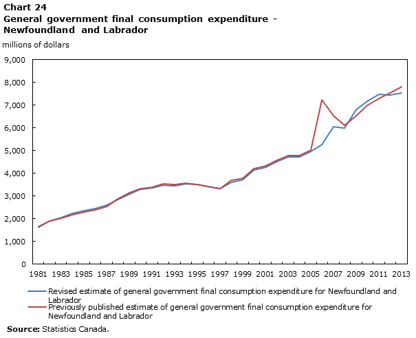
Description for Chart 24
The title of the graph is "Chart 24 General government final consumption expenditure - Newfoundland and Labrador."
This is a line chart.
There are in total 33 categories in the horizontal axis. The vertical axis starts at 0 and ends at 9,000 with ticks every 1,000 points.
There are 2 series in this graph.
The vertical axis is "millions of dollars."
The units of the horizontal axis are years from 1981 to 2013.
The title of series 1 is "Revised estimate of general government final consumption expenditure for Newfoundland and Labrador."
The minimum value is 1,654 occurring in 1981.
The maximum value is 7,545 occurring in 2013.
The title of series 2 is "Previously published estimate of general government final consumption expenditure for Newfoundland and Labrador."
The minimum value is 1,628 occurring in 1981.
The maximum value is 7,811 occurring in 2013.
| Year | Revised estimate of general government final consumption expenditure for Newfoundland and Labrador | Previously published estimate of general government final consumption expenditure for Newfoundland and Labrador |
|---|---|---|
| 1981 | 1,654 | 1,628 |
| 1982 | 1,887 | 1,892 |
| 1983 | 2,044 | 2,032 |
| 1984 | 2,223 | 2,187 |
| 1985 | 2,344 | 2,299 |
| 1986 | 2,432 | 2,389 |
| 1987 | 2,589 | 2,537 |
| 1988 | 2,833 | 2,866 |
| 1989 | 3,078 | 3,136 |
| 1990 | 3,296 | 3,336 |
| 1991 | 3,359 | 3,394 |
| 1992 | 3,485 | 3,527 |
| 1993 | 3,452 | 3,497 |
| 1994 | 3,541 | 3,573 |
| 1995 | 3,500 | 3,511 |
| 1996 | 3,410 | 3,422 |
| 1997 | 3,313 | 3,315 |
| 1998 | 3,589 | 3,687 |
| 1999 | 3,716 | 3,794 |
| 2000 | 4,133 | 4,206 |
| 2001 | 4,271 | 4,330 |
| 2002 | 4,511 | 4,565 |
| 2003 | 4,715 | 4,772 |
| 2004 | 4,734 | 4,788 |
| 2005 | 4,975 | 5,029 |
| 2006 | 5,273 | 7,248 |
| 2007 | 6,042 | 6,540 |
| 2008 | 6,004 | 6,102 |
| 2009 | 6,813 | 6,530 |
| 2010 | 7,169 | 7,003 |
| 2011 | 7,479 | 7,296 |
| 2012 | 7,458 | 7,545 |
| 2013 | 7,545 | 7,811 |
| Source: Statistics Canada | ||
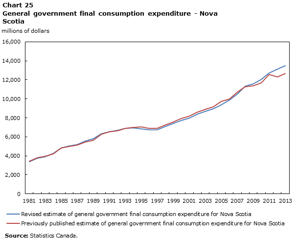
Description for Chart 25
The title of the graph is "Chart 25 General government final consumption expenditure - Nova Scotia."
This is a line chart.
There are in total 33 categories in the horizontal axis. The vertical axis starts at 0 and ends at 16,000 with ticks every 2,000 points.
There are 2 series in this graph.
The vertical axis is "millions of dollars."
The units of the horizontal axis are years from 1981 to 2013.
The title of series 1 is "Revised estimate of general government final consumption expenditure for Nova Scotia."
The minimum value is 3,378 occurring in 1981.
The maximum value is 13,473 occurring in 2013.
The title of series 2 is "Previously published estimate of general government final consumption expenditure for Nova Scotia."
The minimum value is 3,434 occurring in 1981.
The maximum value is 12,648 occurring in 2013.
| Year | Revised estimate of general government final consumption expenditure for Nova Scotia | Previously published estimate of general government final consumption expenditure for Nova Scotia |
|---|---|---|
| 1981 | 3,378 | 3,434 |
| 1982 | 3,746 | 3,801 |
| 1983 | 3,893 | 3,938 |
| 1984 | 4,280 | 4,220 |
| 1985 | 4,834 | 4,825 |
| 1986 | 5,023 | 4,999 |
| 1987 | 5,216 | 5,127 |
| 1988 | 5,534 | 5,473 |
| 1989 | 5,802 | 5,677 |
| 1990 | 6,331 | 6,288 |
| 1991 | 6,541 | 6,516 |
| 1992 | 6,676 | 6,662 |
| 1993 | 6,885 | 6,903 |
| 1994 | 6,924 | 6,995 |
| 1995 | 6,867 | 7,061 |
| 1996 | 6,718 | 6,912 |
| 1997 | 6,717 | 6,877 |
| 1998 | 7,097 | 7,248 |
| 1999 | 7,389 | 7,552 |
| 2000 | 7,741 | 7,927 |
| 2001 | 7,964 | 8,196 |
| 2002 | 8,386 | 8,573 |
| 2003 | 8,699 | 8,916 |
| 2004 | 8,952 | 9,174 |
| 2005 | 9,377 | 9,742 |
| 2006 | 9,906 | 10,006 |
| 2007 | 10,515 | 10,695 |
| 2008 | 11,305 | 11,260 |
| 2009 | 11,569 | 11,395 |
| 2010 | 12,073 | 11,671 |
| 2011 | 12,722 | 12,566 |
| 2012 | 13,117 | 12,316 |
| 2013 | 13,473 | 12,648 |
| Source: Statistics Canada | ||
Household disposable income by province and territory was revised downward for all provinces and territories as part of this comprehensive revision. The downward revision was due to the change in the treatment of pensions in the provincial and territorial economic accounts. Within the provincial and territorial accounts’ household sector table, household payments to pension plans are now shown explicitly as a transfer to financial corporations. This flow represents the pension entitlements earned by households during the period, and which are placed into a pension fund. Similarly, pension funds received by households (pensioners) are shown as a transfer received from the pension fund. On average, the pension payments (transfers to financial corporations) are greater than the pension receipts (transfers from financial corporations) resulting in a downward revision to household disposable income for all provinces and territories. This new treatment aligns with the international standard on recording household disposable income.
| Province or territory | Revised estimate of the average level of household disposable income (1981 to 2013) | Previously published estimate of the average level of household disposable income (1981 to 2013) | Revised estimate of the average level of household disposable income (1981 to 2013) as a share of the previously published estimate |
|---|---|---|---|
| millions of dollars | percent | ||
| Newfoundland and Labrador | 8,112 | 8,631 | 93.99 |
| Prince Edward Island | 2,079 | 2,233 | 93.10 |
| Nova Scotia | 14,684 | 16,030 | 91.60 |
| New Brunswick | 11,477 | 12,296 | 93.34 |
| Quebec | 119,325 | 126,529 | 94.31 |
| Ontario | 222,454 | 232,836 | 95.54 |
| Manitoba | 18,995 | 20,223 | 93.93 |
| Saskatchewan | 17,083 | 17,839 | 95.76 |
| Alberta | 66,857 | 69,148 | 96.69 |
| British Columbia | 72,837 | 76,234 | 95.54 |
| Yukon | 685 | 737 | 92.94 |
| Northwest TerritoriesNote 1 Table 15 | 1,344 | 1,409 | 95.39 |
| NunavutNote 1 Table 15 | 740 | 782 | 94.63 |
|
|||
While disposable income was revised downward, there was little impact on the saving rate by province and territory. This is because a new flow has been added to the provincial and territorial household sector account, after the calculation of household disposable income, called the ‘change in pension entitlements’. This new flow represents the difference between what households pay into pension funds and what they receive. The reason this difference is added back into the household sector’s account is because, although the pension fund received the income from households, the income does represent a pre-determined source of saving for households and therefore needs to be included in the measure of household saving. Why is this income not included in disposable income? One way to answer this is by examining the definition of household disposable income. Household disposable income represents the income available to households to use for consuming or saving. If we include the ‘pension’ saving in household disposable income, we would be overstating their available funds for consumption since these funds have already been set aside as saving.
9. Conclusion
With the 2015 comprehensive revision of the Canadian System of Macroeconomic Accounts, Statistics Canada has taken another step towards fuller compliance with the international macroeconomic accounting standard—the 2008 System of National Accounts and has updated a number of underlying methodologies and data sources, improving the quality and detail available for the user community. As is the case in other G20 countries, improvements can still be made to fully align Canada’s macroeconomic accounts with recommended standards and ensure comparability in an evolving global economy. As such, Statistics Canada is considering further improvements targeted for publication in 2018. Planned changes will be communicated in advance to allow time for adjustment to economic models and analysis. These more frequent updates ensure that the Canadian System of Macroeconomic accounts continues to reflect the ever-changing Canadian and International economic environment.
- Date modified: