Canadian Community Health Survey (CCHS) – Annual component

User guide 2009
Microdata files

1.0 Introduction
2.0 Background
3.0 CCHS redesign in 2007
4.0 Content structure of the CCHS
5.0 Sample Design
6.0 Data Collection
7.0 Data Processing
8.0 Weighting
9.0 Data Quality
10.0 Guidelines for tabulation, analysis and release
11.0 Approximate sampling variability tables
12.0 Microdata files: description, access and use
Appendix A
Appendix B
Appendix C
Appendix D
Appendix E

1.0 Introduction

The Canadian Community Health Survey (CCHS) is a cross–sectional survey that collects information related to health status, health care utilization and health determinants for the Canadian population. It surveys a large sample of respondents and is designed to provide reliable estimates at the health region level. In 2007, major changes were made to the CCHS design. Data is now collected on an ongoing basis with annual releases, rather than every two years as was the case prior to 2007. The survey’s objectives were also revised and are as follows:

• support health surveillance programs by providing health data at the national, provincial and intra–provincial levels;
• provide a single data source for health research on small populations and rare characteristics;
• timely release of information easily accessible to a diverse community of users; and
• create a flexible survey instrument that includes a rapid response option to address emerging issues related to the health of the population.

Details of the other redesign changes are provided in section 3.

The CCHS data is always collected from persons aged 12 and over living in private dwellings in the 121 health regions covering all provinces and territories. Excluded from the sampling frame are individuals living on Indian Reserves and on Crown Lands, institutional residents, full–time members of the Canadian Forces, and residents of certain remote regions. The CCHS covers approximately 98% of the Canadian population aged 12 and over.

The purpose of this document is to facilitate the manipulation of the CCHS microdata files and to describe the methodology used. The CCHS produces three types of microdata files: master files, share files and public use microdata files (PUMF). The characteristics of each of these files are presented in this guide. The PUMF is released every two years and contains two years of data. The next PUMF file will be released in 2011 and will include the data collected for the years 2009 and 2010.

Any questions about the data sets or their use should be directed to:

Electronic Products Help Line: 1–800–949–9491

For custom tabulations or general data support:
Client Custom Services, Health Statistics Division: 613–951–1746
E–mail: hd–ds@statcan.gc.ca

For remote access support: 613–951–1746
E–mail: cchs–escc@statcan.gc.ca
Fax: 613–951–0792

2.0 Background

In 1991, the National Task Force on Health Information cited a number of issues and problems with the health information system. The members felt that data was fragmented; incomplete, could not be easily shared, was not being analysed to the fullest extent, and the results of research were not consistently reaching Canadians.¹

In responding to these issues, the Canadian Institute for Health Information (CIHI), Statistics Canada and Health Canada joined forces to create a Health Information Roadmap. From this mandate, the Canadian Community Health Survey (CCHS) was conceived. The format, content and objectives of the CCHS evolved through extensive consultation with key experts and federal, provincial and community health region stakeholders to determine their data requirements.²

To meet many data requirements, the CCHS had a two–year data collection cycle. Until the redesign in 2007, the first year of the survey cycle, designated by ".1", was a general population health survey, designed to provide reliable estimates at the health region level. The second year of the survey cycle, designated by ".2", had a smaller sample and was designed to provide provincial level results on specific health topics.

New designations for Cycles .1 and .2

As of 2007, the regional component of the CCHS program began being collected on an ongoing basis. To avoid confusion with the health focused surveys, the two components stopped using the “.1” and “.2” designations to distinguish them. Henceforth, the x.1 cycles of the CCHS are designated as "the annual component" of the CCHS. The full title is "The Canadian Community Health Survey – Annual component, 2009" and the short title is simply "CCHS – 2009". The focused content component of the survey remains unchanged. It will continue to examine in greater detail more specific topics or populations. It will be designated by the name of the survey followed by the topic of the themes covered by each survey (example, “Canadian Community Health Survey on Healthy Aging” or “CCHS – Healthy Aging”).

3.0 CCHS Redesign in 2007

Until 2005, the CCHS data were collected every two years over a one year period and released every two years, about six months after the end of the collection period. There were two main objectives for the 2007 CCHS redesign: to address the needs of partners to increase the survey’s content and the frequency of data releases, and to ensure better use of operational resources. For these reasons, the proposed changes to the CCHS design focused on improving the survey’s efficiency and flexibility through ongoing data collection.

Extensive consultations were held across Canada with key experts and federal, provincial and health region stakeholders to gather input on the proposed changes and detailed information on the data requirements and products of the various partners.

Below are the main changes arising from the CCHS redesign:

• In the past, the CCHS data were collected from 130,000 respondents over a 12–month period. Now, data collection takes place on an ongoing basis. The sample, which retains the same size, is divided into 12 two–month collection periods. Each collection period is representative of the population living in the ten Canadian provinces during the two months. For operational reasons, the sample in the territories is representative of their population after 12 months.
   
• The common content component is divided into three: the annual common content (previously referred to as core content), the one year and two-year common content (previously referred to as theme content). The one year common content is asked for one year and re-introduced every two or four years. The two year common content is asked for two years and re-introduced every four years. The two year and one year common content was created to take advantage of the continuous collection approach. The data collection time for this component can be adjusted based on the prevalence of the desired estimates and their geographic level. The annual common content will remain relatively stable over time. At the discretion of the provinces and regions, the optional content can also be adjusted on an annual basis, rather than every two years.
   
• Content and collection changes inevitably impact the dissemination strategy. Previously, data were released every two years. Since 2008, CCHS data are released annually. Every two years, a file combining the two years’ sample (130,000 respondents) is also be released. In addition to these regular files, other special files will be made available when additional content has been collected during collection periods that do not correspond to the standard annual periods, which is January to December.
   
• The annual data collection is divided into six two–month periods. Unlike the previous collection strategy, these periods no longer overlap, which provides more efficient oversight of collection and offers the possibility of changing the collection interface every two months, if necessary.

4.0 Content Structure of the CCHS

In addition to socio–demographic and administrative data, the content of the CCHS includes three components, each of which addresses a different need: annual common content, the two year and one year common content, the optional content component, and the rapid response component. AppendixA lists the modules included in the 2009 questionnaire by component.

The average length of a CCHS interview is estimated at 40 to 45minutes.

Table 4.1 Length of survey by component

CCHS component	Average interview time
Common content Annual One and two-year	30 minutes (20 minutes) (5 minutes)
Optional content	10 minutes
Rapid response content (optional)	2 minutes

4.1 Common content

The CCHS common content component includes questions asked of respondents in all provinces and territories (unless otherwise specified). It is divided into three components: the annual common content, one-year and two year common content.

The annual common content consists of questions asked of all survey respondents. These questions will remain relatively stable in the questionnaire for a period of about six years, unless a major concern is raised about quality.

The one year and two-year common content (previously called theme content) comprises questions related to a specific topic. Combined, the two year and one year common content take about 10 minutes of the interview time. Modules comprising this content type could be reintroduced in the survey every two, four or six years, if required. This component enables CCHS to better plan its content in the medium term.

Some of the modules in the one year common content may be asked of a sub sample of respondents if the objective of these questions is to provide reliable data at the national or provincial level, rather than at the health region level. This approach is used to minimize the related response burden and costs.

4.2 Optional content

The optional content component gives health regions the opportunity to select content that addresses their provincial or regional public health priorities. The optional content is selected from a long list of modules available for inclusion in the CCHS. The content modules selected by a region are asked only of residents in the regions that selected these modules. In reality, since 2005 (cycle 3.1), the regions and provinces have opted to coordinate the optional content selected in order to ensure a uniform selection of optional modules provincially. The optional content may vary annually depending on needs and must be reviewed every two years.

It should be noted that, unlike the modules included in the common content, the resulting data from the optional content modules is not easily generalized across Canada³.

Appendix B presents the selection results of the optional content for the current year by province of residence.

4.3 Rapid response content

The rapid response component is offered on a cost–recovery basis to organizations interested in obtaining national estimates on an emerging or specific topic related to the health of the population. The rapid response content takes a maximum of two minutes of interview time. The questions appear in the questionnaire for a single collection period (two months) and are asked of all CCHS respondents during that period.

4.4 Content included in data files

The survey produces different data files:

• one year reference period
• combined two years reference periods and
• one year sub-sample data files.

Table 4.2 provides clarification about the data files available for the 2009 and 2010 CCHS.

One year data files

The survey produces data files every year. In June 2010, an annual file based on the 2009 reference period has been released. It includes respondents from the 2009 data collection and variables from the common annual content, common one year content, common two year content as well as optional content.

Two year data files

Every two years, a file combining the most recent two years is released. The last combined file was released in 2009 and contained data for 2007 and 2008. The next two years data file will be released in 2011 and will include 2009 and 2010 reference year data .

The two-year data file includes all respondents and the questions that were in the survey over the two year reference period. Unless otherwise specified, it is the question component from the common annual and two-year content and selected optional content over the two year period. The one-year common content and optional content selected for one year only are not available in the two-year data file.

Sub-sample data files

Any modules collected from a sub-sample of the population will continue to be disseminated in separate files. These files include the annual and one year common content collected from a sub-sample of respondents.

Table 4.2 Content components included in 2009 and 2010 data files

Files		Annual common content	2009 one year common content1	2010 one year common content2	2009-2010 two-year common content	Optional content3
2009	Main Sub-sample (2 modules)	Yes Yes	No Yes	N/A N/A	Yes No	Yes No
2010	Main	Yes	N/A	Yes	Yes	Yes
2009-2010	Main	Yes	No	No	Yes	Yes
1 The 2009 annual common content was comprised of two modules (Access to health care services and Waiting times) which were all asked to a sub-sample of respondents. 2 The 2010 annual common content will include a group of modules related to chronic disease screening. 3Optional content will be included in the 2009-2010 data file (to be released in 2011) if it is asked of respondents in a province during the two year period. Otherwise, it will only be included in the file of the year in which it was collected. Note that if an annual common content module from one year is selected for the optional content of a jurisdiction during the second year, the module will be included in the two-year data file and will be processed as optional content.

5.0 Sample design

5.1 Target population

The CCHS targets persons aged 12 years and older who are living in private dwellings in the ten provinces and three territories. Persons living on Indian Reserves or Crown lands, those residing in institutions, full–time members of the Canadian Forces and residents of certain remote regions are excluded from this survey. The CCHS covers approximately 98% of the Canadian population aged 12 and older.

5.2 Health regions

For administrative purposes, each province is divided into health regions (HR) and each territory is designated as a single HR. Statistics Canada is sometimes asked to make minor changes to the boundaries of some of the HRs to correspond to the geography of the Census, or to better account for the health data needs determined by the new geographic boundaries. For CCHS 2008, data was collected in 118 HRs in the ten provinces, as well as to one HR per territory, totalling 121 HRs (Appendix C).

5.3 Sample size and allocation

To provide reliable estimates for each HR given the budget allocated to the CCHS component, it was determined that the survey should consist of a sample of nearly 130,000 respondents over a period of 2 years. Although producing reliable estimates for each HR was a primary objective, the quality of the estimates for certain key characteristics at the provincial level was also deemed important. Therefore, the sample allocation strategy, consisting of three steps, gave relatively equal importance to the HRs and the provinces. In the first step, a minimum size of 500 respondents per HR was imposed. This is considered the minimum for obtaining a reasonable level of data quality. However, due to response burden, a maximum sampling fraction of 1 out of 20 dwellings was imposed to avoid sampling too many dwellings in smaller regions also targeted by other surveys. Note that very few HRs have a size lower than 500 due to limit of the sampling fraction. In this first step, 60,350 units were allocated in total. The second step involves allocating the rest of the available sample by using an allocation proportional to the population size by province. The total sample size by province is therefore the sum of the sizes established by the two first steps. This sample allocation strategy was used for CCHS 3.1 and the sample sizes have remained mainly the same since then. The sample was then divided evenly between the 2 collection years. Table 5.1 gives the annual sample size for 2009.

Table 5.1 Number of health regions and targeted sample sizes by province/territory, 2009

Province	Number of HRs	Total sample size (targeted)
Newfoundland and Labrador	4	2,005
Prince Edward Island	3	1,001
Nova Scotia	6	2,520
New Brunswick	7	2,575
Quebec	16	12,144
Ontario1	36	22,207
Manitoba	10	3,750
Saskatchewan	11	3,860
Alberta	9	6,100
British Columbia	16	8,050
Yukon	1	600
Northwest Territories	1	600
Nunavut	1	350
Canada	121	65,762
1The sample size for Ontario includes the buy–in extra sample by LHIN. The initial sample size for Ontario before the buy–in was 20,880 units (refer to section 5.7 for further details).

In the third step, the provincial sample was allocated among its HRs proportionally to the square root of the estimated population in each HR. This three–step approach gives sufficient sample for each HR with minimal disturbance to the proportionality of the allocation by province.

Note that the three territories were not part of the above allocation strategy as they were dealt with separately. In total, for 2009, 600 sample units were allocated to the Yukon, 600 to the Northwest Territories and 350 to Nunavut. These sizes are determined according to the available budget. The sample allocation for the territories is done proportionally to the population sizes of the strata. The strata used were the same as those defined by the Labour Force Survey (LFS), which group together communities (For more details, see section 5.4.1).

The sample was then equally divided in 2 in order to obtain the same sample sizes between the area frame sample and the list frame sample for each HR⁴, as described in the next section. We should finally mention that the size of the samples taken from each frame was increased before data collection in order to account for the anticipated out–of–scope and non–response rates based on the rates obtained in previous CCHS cycles. The sample sizes by HR and frame are provided in Appendix D.

5.4 Frames, household sampling strategies

CCHS 2009 used three sampling frames to select the sample of households: 49% of the sample of households came from an area frame, 50% came from a list frame of telephone numbers and the remaining 1% came from a Random Digit Dialling (RDD) sampling frame.

5.4.1 Sampling of households from the area frame

The CCHS used the area frame designed for the Canadian Labour Force Survey (LFS) as a sampling frame. The sampling plan of the LFS is a multistage stratified cluster design in which the dwelling is the final sampling unit⁵. In the first stage, homogeneous strata are formed and independent samples of clusters are drawn from each stratum. In the second stage, dwelling lists are prepared for each cluster and dwellings, or households, are selected from these lists.

For the purpose of the LFS plan, each province is divided into three types of regions: major urban centres, cities, and rural regions. Geographic or socio–economic strata are created within each major urban centre. Within the strata, between 150 and 250 dwellings are grouped together to create clusters. Some urban centres have separate strata for apartments or for census Dissemination Areas (DA) to pinpoint households with high income, immigrants and aboriginals. In each stratum, six clusters or residential buildings (sometimes 12 or 18 apartments) are chosen by a random sampling method with a probability proportional to size (PPS), the size of which corresponds to the number of households. The number six is used throughout the sample design to allow for one sixth of the LFS sample to be rotated each month.

The other cities and rural regions of each province are stratified first on a geographical basis, then according to socio–economic characteristics. In the majority of strata, six clusters (usually census DAs) are selected using the PPS method. Some geographically isolated urban centres are covered by a three–stage sampling design. This type of sampling plan is used for Quebec, Ontario, Alberta and British Columbia.

Once the new clusters are listed, the sample is obtained using a systematic sampling of dwellings. The sample size for each systematic sample is called the “yield”. Table 5.2 gives an overview of the types of PSUs used in the LFS sample and the yield predicted by systematic sample. As the sampling rates are determined in advance, there is frequently a difference between the expected sample size and the numbers that are obtained. The yield of the sample, for example, is sometimes excessive. This can particularly happen in sectors where there is an increase in the number of dwellings due to new construction. To reduce the cost of collection, an excessive output is corrected by eliminating, from the beginning, a part of the units selected and by modifying the weight of the sample design. This change is dealt with during weighting.

Table 5.2 Major first–stage units, sizes and yields

Area	Primary Sampling Unit (PSU)	Size (households per PSU)	Yield (sampled households)
Toronto, Montreal, Vancouver	Cluster	150–250	6
Other cities	Cluster	150–250	8
Most rural areas / small urban centres	Cluster	100–250	10

Due to the specific of the CCHS, some modifications had to be incorporated in this sampling strategy. To obtain an annual sample of 33,000 respondents for CCHS 2009, close to 48,000 dwellings had to be selected from the area frame to account for vacant dwellings and non–responding households. Each month, the LFS design provides approximately 60,000 dwellings distributed across the various economic regions in the ten provinces, whereas the CCHS 2009 required 48,000 dwellings distributed across the HRs, which have different geographic boundaries from those of the LFS economic regions. Overall, the CCHS 2009 required a lower number of dwellings than those generated by the LFS selection mechanism, which corresponds to an adjustment factor of 0.80 (48,000/60,000). However, since the adjustment factors varied from 0.3 to 3.0 at the HR level, certain adjustments were required.

The changes made to the selection mechanism in the regions varied depending on the size of the adjustment factors. For HRs that had a factor smaller than or equal to 1, the number of PSUs selected was reduced if necessary. For example, if the factor was 0.5 then only 3 PSUs were selected in each stratum instead of the usual number of 6 PSUs. For those HRs with a factor greater than 1 but smaller than or equal to 2, the sampling process of dwellings within a PSU was repeated for a subset of the selected PSUs that were part of the same HR. For example, if the factor was 1.6 then the selection of dwellings within a PSU was repeated for 4 of the 6 PSUs in all strata of that HR. When it was necessary to have a repeated selection of dwellings within a PSU and there were no more dwellings available in that PSU, then another PSU was selected. When the factor was greater than 2, the sampling process of dwellings was repeated among other PSUs that were part of the same HR⁶.

Finally, when the number of dwellings available in the selected PSUs was greater than the requested number of dwellings for a given HR, a sub–sample of dwellings was selected. This process is called ‘stabilization’.

Sampling of households from the area frame in the three territories

For operational reasons, the LFS area frame sample design for the three territories is different. For each territory, in–scope communities are grouped into strata based on various characteristics (population, geographical information, proportion of Inuit and/or Aboriginal persons, and median household income). The LFS defined five design strata in the Yukon, ten in the Northwest Territories and six in Nunavut. The first stage of selection consisted of randomly selecting one community with a probability proportional to population size within each design stratum. Then, within the selected community, a household sampling strategy was put in place identically to the one described above. The CCHS selected its sample from the same communities sampled by the LFS, while ensuring that different dwellings were selected. If too many or too few dwellings were available for a community within a stratum, the LFS chose another community for the CCHS.

It is worth mentioning that the frame for the CCHS 2009 covered 90% of the private households in the Yukon, 97% in the Northwest Territories and 71% in Nunavut⁷.

5.4.2 Sampling of households from the list frame of telephone numbers

With the exception of 5 HRs (the two RDD only HRs and the three territories), the list frame of telephone numbers was used in all HRs to complement the area frame. The list frame consists of the Canada Phone directory which is an external administrative database of names, addresses and telephone numbers from telephone directories in Canada updated every six months. It was linked to administrative conversion files to obtain postal codes, and these were mapped to HRs to create list frame strata. There was one list frame stratum per HR. Within each stratum, the required number of telephone numbers was selected using a simple random sampling process from the list. As for the RDD frame, additional telephone numbers were selected to account for the numbers not in service or out–of–scope.

It is important to mention that the undercoverage of the list frame is higher than the one for the RDD as unlisted numbers do not have a chance of being selected. Nevertheless, as the list frame is always used as a complement to the area frame, the impact of the undercoverage of the list frame is minimal and is dealt with during weighting.

5.4.3 Sampling of households from the RDD frame of telephone numbers

In four HRs, a Random Digit Dialing (RDD) sampling frame of telephone numbers was used to select a sample of households. The sampling of households from the RDD frame used the Elimination of Non–Working Banks (ENWB) method, a procedure adopted by the General Social Survey⁸. A bank of one hundred telephone numbers (the first eight digits of a ten–digit telephone number) is considered to be non–working if it does not contain any residential telephone numbers. At first, the frame consists of a list of all possible banks and, as non–working banks are identified, they are eliminated from the frame. It should be noted that these banks are eliminated only when there is evidence from various sources that they are non–working. When there is no information about a bank it is left on the frame. The Canada Phone Directory and telephone companies’ billing address files were used in conjunction with various internal administrative files to eliminate non–working banks.

Using available geographic information (postal codes), the banks on the frame were regrouped to create RDD strata to encompass, as closely as possible, the HR areas. Within each RDD stratum, a bank was randomly chosen and a number between 00 and 99 was generated at random to create a complete, ten–digit telephone number. This procedure was repeated until the required number of telephone numbers within the RDD stratum was reached. Frequently, the number generated is not in service or is out–of–scope, and therefore, many additional numbers must be generated to reach the targeted sample size. This success rate varies from region to region. Within the CCHS, the success rates ranged from 25% to 50% among the four HRs which required the use of the RDD frame.

5.5 Sample allocation over the collection period

In order to balance interviewer workload and to minimize possible seasonal effects on estimates of certain key characteristics such as physical activity, the initial sample of dwellings / telephone numbers was allocated at random, within each HR, over a two–month data collection period.

In the area frame, each start selected within each HR was randomly assigned to a collection period accounting for a number of constraints related to field operations or weighting, while maintaining a uniform size for each period. For example, a sample that is representative of the Canadian population is ensured every six months by ensuring that the dwelling sample covers all LFS strata during this period.

For the lists of telephone numbers, independent samples were selected in each collection period. This strategy ensures that each sample is representative of the Canadian population that is within the scope of the survey in each two months.

5.6 Sampling of interviewees

As was done for the previous cycles, the selection of individual respondents was designed to ensure over–representation of youths (12 to 19). The selection strategy that was adopted accounted for user needs, cost, design efficiency, response burden and operational constraints. One person is selected per household using varying probabilities taking into account the age and the household composition. The selection probabilities resulted from simulations using various parameters in order to determine the optimal approach without causing extreme sampling weights.

Table 5.3 gives the selection weight multiplicative factors used to determine the probabilities of selection of individuals in sampled households by age group. For example, for a three–person household (two adults of age 45 to 64 and one 15–year–old), the teenager would have 6.5 times more chance of being selected compared to the adults. To avoid extreme sampling weights, there is one exception to this rule: if the size of the household is greater than or equal to 5 or if the number of 12–19 year olds is greater than or equal to 3 then the selection weight multiplicative factor equals 1 for each individual in the household. Consequently, all people in that household have the same probability of being selected.

Table 5.3 Selection weight multiplicative factors for the person–level sampling strategy by age

	Selection Weight Multiplicative Factors
Age	12 to 19	20 to 29	30 to 44	45 to 64	65+
Factor	65	25	20	10	10

5.7 Supplementary buy–in sample in three health regions in Ontario

The province of Ontario requested a sample increase in order to produce estimates at the Local Health Integrated Network (LHIN) geography level. Ontario contains 14 LHIN. The CCHS sample was increased in order to obtain a minimum size of 2,000 per LHIN over a period of 2 years. As the HR and LHIN boundaries intersect each other, the stratification level used was the HR–LHIN overlap. The preliminary sample sizes allotted by HR are therefore preserved. In cases where the HR allocation prevented the sample from reaching sizes of 2,000 per LHIN, the sample was then increased, and was allocated proportionally to the size of the population within the HR–LHIN overlap. Table 5.4 provides the sample sizes of targeted respondents by LHIN for 2009.

Table 5.4 Targeted respondents by Local Health Integrated Network (LHIN), CCHS 2008.

LHIN	Targeted respondents
01–Erie St. Clair	1,550
02–South West	2,561
03–Waterloo Wellington	1,242
04–Hamilton Niagara Haldimand Brant	2,597
05–Central West	1,069
06–Mississauga Halton	1,115
07–Toronto Central	1 081
08–Central	1,411
09–Central East	2,108
10–South East	1,313
11–Champlain	2,057
12–North Simcoe Muskoka	1,050
13–North East	1,990
14–North West	1,063
Ontario	22,207

The total sample size of the HR–LHIN overlapping areas was then allocated equally between the list frame and the area frame. The usual sample selection procedures within each frame were then applied to the total sample. The additional sample was included as part of the full CCHS sample. Sample sizes by Local Health Integrated Network and frame are given in Appendix D.

5.8 Sub-sample for the Health Services Access Survey (HSAS)

A sub-sample of the CCHS was taken to obtain additional information on the services and access to health care. The survey covers the same population as the CCHS, except for the territories and persons less than 15 years of age.

The budget allocated to this sub-sample was similar to the previous survey, at nearly 48,000 respondents, which ensured that reliable estimates could be produced at the provincial level. The sample allocation was conducted similar to that in CCHS 2007. However, the sample was not increased in PEI, so only the 1,001 units available from the CCHS 2009 sample were used. Here are the sample sizes for the HSAS 2009 survey.

Table 5.5: Sample sizes of CCHS 2009 and the HSAS 2009 by province.

	Sample Size
Province	CCHS 2009	HSAS 2009
Newfoundland and Labrador	2,005	2,005
Prince Edward Island	1,001	1,001
Nova Scotia	2,520	2,520
New Brunswick	2,575	2,575
Quebec	12,114	4,600
Ontario	22,207	22,207
Manitoba	3,750	3,200
Saskatchewan	3,806	3,200
Alberta	6,100	3,600
British Columbia	8,050	4,000
CANADA	64,212	48,908

Once the size is defined by province, the sample was allocated by HR proportionally to the HR population size, which thus ensured a better sample allocation by province while accounting for the stratification of CCHS by HR. In provinces where the sample size by HR was insufficient, a power allocation with a power less than 1 had to be used. A power of 0.9 was used in Alberta and British Columbia, whereas a power of 0.55 had to be used in Manitoba and Saskatchewan, which made the design less optimal. For the other provinces, no allocation by HR was necessary since the entire CCHS sample was used.

Finally, the sample was allocated evenly between the list frame and the area frame. The size was also increased to account for out-of-scope units, and for the predicted non-response rate. Where possible, the size was once again inflated to account for the population not covered by HSAS (12-14 year-olds) and proxy interviews that were not accepted in HSAS. Final sample sizes and the expected number of respondents by province and frame are given in Appendix D.

Sample selection was performed independently in each collection period based on the CCHS samples. A equally sub-sample of dwellings or telephone numbers was selected randomly in each HR every collection period.

6.0 Data collection

6.1 Computer–assisted interviewing

Between January and December 2009, a total of 61,679 valid interviews were conducted using computer assisted interviewing (CAI). Approximately half the interviews were conducted in person using computer assisted personal interviewing (CAPI) and the other half were conducted over the phone using computer assisted telephone interviewing (CATI).

CAI offers two main advantages over other collection methods. First, CAI offers a case management system and data transmission functionality. This case management system automatically records important management information for each attempt on a case and provides reports for the management of the collection process. CAI also provides an automated call scheduler, i.e. a central system to optimise the timing of call–backs and the scheduling of appointments used to support CATI collection.

The case management system routes the questionnaire applications and sample files from Statistics Canada’s main office to regional collection offices (in the case of CATI) and from the regional offices to the interviewers laptops (for CAPI). Data returning to the main office takes the reverse route. To ensure confidentiality, the data is encrypted before transmission. The data are then unencrypted when they are on a separate secure computer with no remote access.

Second, CAI allows for custom interviews for every respondent based on their individual characteristics and survey responses. This includes:

• questions that are not applicable to the respondent are skipped automatically
• edits to check for inconsistent answers or out–of–range responses are applied automatically and on–screen prompts are shown when an invalid entry is recorded. Immediate feedback is given to the respondent and the interviewer is able to correct any inconsistencies.
• question text, including reference periods and pronouns, is customised automatically based on factors such as the age and sex of the respondent, the date of the interview and answers to previous questions.

6.2 CCHS application development

The CCHS uses two separate CAI applications to collect data, one for telephone interviews (CATI) and one for personal interviews (CAPI). This was done in order to customise each applications’ functionality to the type of interview being conducted. Each application consisted of entry, health content (known as the C2), and exit components.

Entry and exit components contain standard sets of questions designed to guide the interviewer through contact initiation, collection of important sample information, respondent selection and determination of cases status. The C2 consists of the health modules themselves and made up the bulk of the applications. This includes common modules asked of all respondents and optional modules which differed by health region. Each application underwent three stages of testing: block, integrated and end to end.

Block level testing consists of independently testing each content module or “block” to ensure skip patterns, logic flows and text, in both official languages, are specified correctly. Skip patterns or logic flows across modules are not tested at this stage as each module is treated as a stand alone questionnaire. Once all blocks are verified by several testers they are added together along with entry and exit components into integrated applications. These newly integrated applications are then ready for the next stage of testing.

Integrated testing occurs when all of the tested modules are added together, along with the entry and exit components, into an integrated application. This second stage of testing ensures that key information such as age and gender are passed from the entry to the C2 and exit components of the applications. It also ensures that variables affecting skip patterns and logic flows are correctly passed between modules within the C2. Since, at this stage the applications essentially function as they will in the field, all possible scenarios faced by interviewers are simulated to ensure proper functionality. These scenarios test various aspects of the entry and exit components including, establishing contact, collecting contact information, determining whether a case is in scope, rostering households, creating appointments and selecting respondents. The applications are also tested to ensure that during an interview, correct modules are triggered reflecting health region optional content selections.

End to end testing occurs when the fully integrated applications are placed in simulated collection environment. The applications are loaded onto computers that are connected to a test server. Data is then collected, transmitted and extracted in real time, exactly as it would be done in the field. This last stage of testing allows for the testing of all technical aspects of data input, transmission and extraction for each of the CCHS applications. It also provided a final chance of finding errors within the entry, C2 and exit components.

6.3 Interviewer training

Project managers, senior interviewers and interviewers from regional collection offices were sent self study training packages before the start of collection. These packages were prepared by the CCHS project team and were used by existing experienced CCHS interviewers to reinforce their previous training. Project managers and senior interviewers also conducted customised training sessions for new CCHS interviewing staff as needed. There were also specific training sessions to deal with various topics related to CCHS collection on a monthly basis.

The focus of the training sessions were to get interviewers comfortable using the CCHS 2009 applications, and familiarise interviewers with survey content and to introduce interviewers to interviewing procedures specific to the CCHS. The training focused on:

• goals and objectives of the survey including a focus on the survey redesign
• survey methodology
• application functionality
• review of the questionnaire content and exercises with an emphasis on significant content changes
• interviewer techniques for maintaining response – complete exercises to minimise non–response
• use of mock interviews to simulate difficult situations and practise potential non–response situations
• survey management
• transmission procedures

One of the key aspects of the training was a focus on minimizing non–response. Exercises to minimise non–response were prepared for interviewers. The purpose of these exercises was to have the interviewers practice convincing reluctant respondents to participate in the survey. There was also a series of refusal avoidance workshops given to the senior interviewers responsible for refusal conversion in each regional collection office.

6.4 The interview

Sample units selected from the telephone list and RDD (Random Digit Dialling) frames were interviewed from centralised call centres using CATI. The CATI interviewers were supervised by a senior interviewer located in the same call centre. Units selected from the area frame were interviewed by decentralised field interviewers using CAPI. While in some situations field interviewers were permitted to complete some or part of an interview by telephone, three–quarters (74.1%) of these interviews were conducted exclusively in person. CAPI interviewers worked independently from their homes using laptop computers and were supervised from a distance by senior interviewers. The variable SAM_TYP on the microdata files indicates whether a case was selected from the area frame (CAPI) or from the telephone or RDD frame (CATI).

In all selected dwellings, a knowledgeable household member was asked to supply basic demographic information on all residents of the dwelling. One member of the household was then selected for a more in–depth interview, which is referred to as the C2 Interview.

CAPI interviewers were trained to make an initial personal contact with each sampled dwelling. In cases where this initial visit resulted in non–response, telephone follow–ups were permitted. The variable ADM_N09 on the microdata files indicates whether the interview was completed face–to–face, by telephone or using a combination of the two techniques.

To ensure the quality of the data collected, interviewers were instructed to make every effort to conduct the interview with the selected respondent in privacy. In situations where this was unavoidable, the respondent was interviewed with another person present. Flags on the microdata files indicate whether somebody other than the respondent was present during the interview (ADM_N10) and whether the interviewer felt that the respondent’s answers were influenced by the presence of the other person (ADM_N11).

To ensure the best possible response rate attainable, many practices were used to minimise non–response, including:

a) Introductory letters
Before the start of each collection period introductory letters explaining the purpose of the survey were sent to the sampled households. These explained the importance of the survey and provided examples of how CCHS data would be used.

b) Initiating contact
Interviewers were instructed to make all reasonable attempts to obtain interviews. When the timing of the interviewer's call (or visit) was inconvenient, an appointment was made to call back at a more convenient time. If requests for appointments were unsuccessful over the telephone, interviewers were instructed to follow–up with a personal visit. If no one was home on first visit, a brochure with information about the survey and intention to make contact was left at the door. Numerous call–backs were made at different times on different days.

c) Refusal conversion
For individuals who at first refused to participate in the survey, a letter was sent from the nearest Statistics Canada Regional Office to the respondent, stressing the importance of the survey and the household's collaboration. This was followed by a second call (or visit) from a senior interviewer, a project supervisor or another interviewer to try to convince respondent of the importance of participating in the survey.

d) Language barriers
To remove language as a barrier to conducting interviews, each of the Statistics Canada Regional Offices recruited interviewers with a wide range of language competencies. When necessary, cases were transferred to an interviewer with the language competency needed to complete an interview.

e) Youth interviews
Interviewers were obliged to obtain verbal permission from parents/guardians to interview youths between the ages of 12 to 15 who were selected for interviews. Several procedures were followed by interviewers to alleviate potential parental concerns and to ensure a completed interview. Interviewers carried with them a card entitled “Note to parents / guardians about interviewing youths for the Canadian Community Health Survey”. This card explained the purpose of collecting information from youth, lists the subjects to be covered in the survey, asks for permission to share and link the obtained information and explains the need to respect a child's right to privacy and confidentiality.

If a parent/guardian asked to see the actual questions; interviewers were instructed to either show the survey questions, or if the interviewer was being conducted by phone, to immediately have the regional office send a copy of the questionnaire.

If privacy could not be obtained to interview the selected youth either in person or over the phone (another person listening in) the interview was coded a refusal. However, for CAPI interviews, if privacy could not be obtained to interview the selected youth, the interviewer was able to propose to the parent/guardian that the interviewer read the questions out loud and the youth enter their answers directly on the computer.

During all interviews conducted with youths, survey questions regarding income and food security were answered by the parent/guardian. These questions were asked at the end of the survey questionnaire, so that when they came up, the parent/guardian could complete the interview.

f) Proxy interviews
In cases where the selected respondent was, for reasons of physical or mental health, incapable of completing an interview, another knowledgeable member of the household supplied information about the selected respondent. This is known as a proxy interview. While proxy interviewees were able to provide accurate answers to most of the survey questions, the more sensitive or personal questions were beyond the scope of knowledge of a proxy respondent. This resulted in some questions from the proxy interview being unanswered. Every effort was taken to keep proxy interviews to a minimum. The variable ADM_PRX indicates whether a case was completed by proxy.

6.5 Field operations

The majority of the 2009 sample was divided into six non–overlapping two–month collection periods. Regional collection offices were instructed to use the first 4 weeks of each collection period to resolve the majority of the sample, with next 4 weeks being used finalise the remaining sample and to follow up on outstanding non–response cases. All cases were to have been attempted by the second week of each collection period.

Sample files were sent approximately two weeks before the start of each collection period to centralised collection offices. A series of dummy cases were included with each CAPI sample. These cases were completed by senior interviewers for the purposes of ensuring that all data transmission procedures were working through the collection cycle. Once, the samples were received, project supervisors were responsible for planning CAPI interviewer assignments. Wherever possible, assignments were generally no larger than 15 cases per interviewer.

Transmission of cases from each of the CATI offices to head office was the responsibility of the regional office project supervisor, senior interviewer and the technical support team. These transmissions were performed nightly and sent all completed cases to Statistics Canada’s head office. Completed CAPI interviews were transmitted daily from the interviewer’s home directly to Statistics Canada’s head office using a secure telephone transmission.

At the end of data collection, a national response rate of 73% was achieved. Complete details regarding the response rates can be found in Appendix E.

6.6 Quality control and collection management

During the 2009 collection year, several methods were used to ensure data quality and to optimize collection. These included using internal measures to verify interviewer performance and the use of a series of ongoing reports to monitor various collection targets and data quality.

A system of validation was used for CAPI cases whereby interviewers had their work validated on a regular basis by the Regional Office. Each collection period, randomly selected cases were flagged in the sample. Regional office managers and supervisors created lists of cases to be validated. These cases were handed to the validation team who then contacted households to verify that a legitimate interview took place. Validation procedures generally occurred during the first few weeks of a collection period to ensure that any issues were detected promptly. Interviewers were provided feedback by their supervisors on a regular basis.

CATI interviewers were also randomly chosen for validation. Validation in the CATI collection offices consisted of senior interviewers monitoring interviews to ensure proper techniques and procedures (reading the questions as worded in the applications, not prompting respondents for answers, etc.) were followed by the interviewer.

A series of reports were produced to effectively track and manage collection targets and to assist in identifying other collection issues.

Cumulative reports were generated at the end of each collection period, showing response, link, share and proxy rates for both the CATI and CAPI samples by individual health region. The reports were useful in identifying health regions that were below collection target levels, allowing the regional offices to focus efforts in these regions.

Using information obtained from the CAI applications, further analysis was done in head office in order to identify interviews that were completed below acceptable time frames. These short interviews were flagged, removed from the microdata and treated as non–response.

7.0 Data processing

7.1 Editing

Most editing of the data was performed at the time of the interview by the computer–assisted interviewing (CAI) application. It was not possible for interviewers to enter out–of–range values and flow errors were controlled through programmed skip patterns. For example, CAI ensured that questions that did not apply to the respondent were not asked.

In response to some types of inconsistent or unusual reporting, warning messages were invoked but no corrective action was taken at the time of the interview. Where appropriate, edits were instead developed to be performed after data collection at Head Office. Inconsistencies were usually corrected by setting one or both of the variables in question to "not stated".

7.2 Coding

Pre–coded answer categories were supplied for all suitable variables. Interviewers were trained to assign the respondent’s answers to the appropriate category.

In the event that a respondent’s answer could not be easily assigned to an existing category, several questions also allowed the interviewer to enter a long–answer text in the “Other–specify” category. All such questions were closely examined in head office processing. For some of these questions, write–in responses were coded into one of the existing listed categories if the write–in information duplicated a listed category. For all questions, the ‘Other–specify’ responses are taken into account when refining the answer categories for future cycles.

7.3 Creation of derived variables

To facilitate data analysis and to minimize the risk of error, a number of variables on the file have been derived using items found on the CCHS questionnaire. Derived variables generally have a "D", "G" or “F” in the fourth character of the variable name. In some cases, the derived variables are straightforward, involving collapsing of response categories. In other cases, several variables have been combined to create a new variable. The Derived Variables Documentation (DV) provides details on how these more complex variables were derived. For more information on the naming convention, please go to Section 12.5.

7.4 Weighting

The principle behind estimation in a probability sample such as CCHS is that each person in the sample "represents", besides himself or herself, several other persons not in the sample. For example, in a simple random 2% sample of the population, each person in the sample represents 50 persons in the population. In the terminology used here, it can be said that each person has a weight of 50.

The weighting phase is a step that calculates, for each person, his or her associated sampling weight. This weight appears on the PUMF, and must be used to derive meaningful estimates from the survey. For example, if the number of individuals who smoke daily is to be estimated, it is done by selecting the records referring to those individuals in the sample having that characteristic and summing the weights entered on those records.

Details of the method used to calculate sampling weights are presented in Section 8.

8.0 Weighting

In order for estimates produced from survey data to be representative of the covered population, and not just the sample itself, users must incorporate the survey weights in their calculations. A survey weight is given to each person included in the final sample, that is, the sample of persons having responded to the survey. This weight corresponds to the number of persons in the entire population that are represented by the respondent.

As described in Section 5, the CCHS has recourse to three sampling frames for its sample selection: an area frame acting as the primary frame and two frames made up of telephone numbers used to complement the area frame. Since only minor differences differentiate the two telephone frames in terms of weighting, they are treated together as one and referred to as being part of the telephone frame.

Depending on the need, one or two frames are used for the selection of the sample within a given health region (HR). When two frames are used, the weighting strategy treats both the area and telephone frames independently to come up with separate household–level weights for each of the frames used. These household–level weights are then combined into a single set of household weights through a step called "integration". After applying person–level selection weights and some further adjustments, this integrated weight becomes the final person–level weight.

8.1 Overview

As mentioned earlier, units from both the area and telephone frames are treated separately up to the integration step. The following sections describe the weighting process for the provinces. Sub–section 8.2 provides details on the weighting strategy for the area frame, while sub–section 8.3 deals with the strategy for the telephone frame. The integration of the two frames is discussed in 8.4. This is followed by the last weighting steps including calibration, where the weights are adjusted to control for seasonality and to match known population totals. These steps are explained in sub–section 8.5.

Although the two frames are used to cover the three territories, the sampling methods used are slightly different from those used in the provinces. These modifications affect the weighting of these three regions substantially, and they are reported in sub–section 8.6.

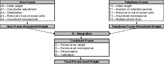
Diagram A presents an overview of the different adjustments that are part of the weighting strategy. A numbering system is used to identify each adjustment and will be used throughout the section. Letters A and T are used as prefixes to refer to adjustments applied to the units on the Area and Telephone frames respectively, while prefix I identifies adjustments applied from the Integration step onwards.

Diagram A Weighting strategy overview

8.2 Weighting of the area frame sample

A0 – Initial weight

The weighting on the area frame sample begins with a weight provided by the Labour Force Survey (LFS). This weight is based on the LFS design since the CCHS area frame sample design is based on the LFS. The LFS design consists of a sample of dwellings within clusters selected from LFS strata. In the initial adjustment, the LFS weight is adjusted to take into consideration the fact that the CCHS selects a sample to be representative of the Health Region. To do so, the CCHS selects a different number of clusters than the LFS and can repeat the sampling of dwellings within the selected clusters. The resulting weight is called A0. For more details about the selection mechanism, as well as a more complete definition of LFS strata and clusters, refer to Statistics Canada (1998)⁹.

A1 – Sub–cluster adjustment

In clusters that experience significant growth, a sub–sampling methodology is used to ensure that the workload of the interviewers is kept at a reasonable level. This can consist of sub–sampling from the selected dwellings, dividing the cluster into sub–clusters, or reclassifying the cluster as a stratum and creating new clusters within the stratum. In all these cases, a sub–sample adjustment is calculated and applied to the CCHS weight. This adjustment is applied to weight A0 to produce weight A1. Again, more information can be found in the LFS documentation (Statistics Canada (1998)).

A2 – Stabilization

In some HRs, the increase of the sample size as described in section 5, results in a larger sample than necessary. Stabilization is used to bring the sample size back down to the desired level. The stabilization process consists of randomly sub–sampling dwellings at the HR level from the dwellings originally selected within each cluster. An adjustment factor representing the effect of this stabilization is calculated in order to adjust the probability of selection appropriately. This factor, multiplied by weight A1, produces weight A2.

A3 – Removal of out–of–scope units

Among all dwellings sampled, a certain proportion is identified during collection as being out–of–scope. Dwellings that are demolished or under construction, vacant, seasonal or secondary, and institutions are examples of out–of–scope cases for the CCHS. These dwellings and their associated weight are simply removed from the sample. This leaves a sample that consists of, and representative of, in–scope dwellings or households. These in–scope dwellings that remain maintain the same weight as in the previous step, which is now called A3.

A4 – Household nonresponse

During collection, a certain proportion of sampled households inevitably result in nonresponse. This usually occurs when a household refuses to participate in the survey, provides unusable data, or cannot be reached for an interview. Weights of the nonresponding households are redistributed to responding households within response homogeneity groups (RHGs). In order to create the response groups, a scoring method based on logistic regression models is used to determine the propensity to respond and these response probabilities are used to divide the sample into groups with similar response properties. The information available for nonrespondents is limited so the regression model uses characteristics such as the collection period and geographic information, as well as paradata or process data, which includes the number of contact attempts, the time/day of attempt, and whether the household was called on a weekend or weekday. Starting in 2008, RHGs were formed within province to better control for provincial totals. An adjustment factor is calculated within each response group as follows:

Weight A3 is multiplied by this factor to produce weight A4 for the responding households. Non–responding households are dropped from the process at this point.

8.3 Weighting of the telephone frame sample

As mentioned earlier, the telephone frame is composed of two frames: a Random Digit Dialling (RDD) frame and a list frame. Only one of the frames can be used within an HR. When the list frame is used, it is always used as a complement to the area frame within the HR. When the RDD frame is used, it is always used as the only frame within the HR. For the purposes of weighting, units coming from the two telephone frames are treated together and therefore are subject to the same adjustments.

The geographical boundaries used to select the sample from the telephone frame do not always conform to the HR geography. Consequently, some units may have been sampled from one HR but the information collected at the time of the interview places them in a neighbouring HR. This is handled in the weighting by applying the first 3 telephone adjustments (T0, T1 and T2) relative to the HR assigned at the time of sample selection. The remaining 2 adjustments (T3 and T4) are applied to the HR based on information collected from the respondent to ensure that all units belong to their correct HR.

T0 –Initial weight

The initial design weight is defined as the inverse of the probability of selection and is computed separately for the RDD and list frame samples since the method of selection differs between these two frames. For the RDD frame, the selection of telephone numbers is done within each RDD stratum. An RDD stratum is an aggregation of area code prefixes (ACP: the first six digits of a 10–digit telephone number), with each ACP containing valid banks of one hundred numbers (see Norris and Paton¹⁰ for more details). Therefore, the probability of selection is the ratio between the number of sampled units and one hundred times the number of banks within the RDD stratum.

For the list frame, telephone numbers are randomly selected among those assigned to the specific HR. The probability of selection corresponds to the ratio of the number of sampled units to the number of telephone numbers on the list within the HR. The ratio is based on the frame available and the number of units selected for the particular two–month collection period. The probability of selection can therefore change depending on sample allocation and frame updates. The inverse of these probabilities represents the initial weight T0.

T1 – Number of collection periods

On the area frame, the entire sample is selected at the beginning of the year. This is in contrast to the telephone frame, where samples are drawn every two months. Each of these samples comes with an initial weight that allows each sample to be representative of the population at the HR level. To ensure that the total sample represents the population only once, an adjustment factor is applied to reduce the weights of each two–month sample. The adjustment factor applied to each two–month sample is equal to the the inverse of the number of samples being combined (i.e. the number of collection periods). Following this adjustment, the entire list frame sample corresponds to the average over the entire combined collection period. The initial weights are multiplied by this adjustment factor to produce weight T1.

T2 – Removal of out–of–scope numbers

Telephone numbers associated with businesses, institutions or other out–of–scope dwellings, as well as numbers not in service or any other non–working numbers are all examples of out–of–scope cases for the telephone frame. Similar to the methods used on the area frame, these cases are simply removed from the process, leaving only in–scope dwellings in the sample. These in–scope dwellings keep the same weight as in the previous step, now called weight T2.

T3 – Household nonresponse

The adjustment applied here to compensate for the effect of household nonresponse is identical to the one applied for the area frame (adjustment A4) although the paradata used does differ because of the differences in collection applications for personal and telephone interviews. The adjustment factor calculated within each class was obtained as follows:

The weight T2 of responding households is multiplied by this factor to produce the weight T3. Nonresponding households are removed from the process at this point.

T4 – Multiple phone lines

Some households can possess more than one residential telephone line. This has an impact on the weighting because these households have a higher probability of being selected. The weights for these households need to be adjusted for the number of residential telephone lines within the household. The adjustment factor represents the inverse of the number of lines in the household. The weight T4 is obtained by multiplying this factor by the weight T3.

8.4 Integration of the telephone and area frames (I1)

This step consists of integrating the weights for households common to the area and telephone frames into a single weight by applying a method of integration¹¹. Those units on the area frame that are not on the telephone frame do not have their weights adjusted. For all others units, an adjustment factor α between 0 and 1 is applied to the weights. The weight of the area frame units is multiplied by this factor α, while the weight of the telephone frame units is multiplied by 1– α. Note that in the case where an HR is covered by only one frame, the adjustment factor is equal to 1. The product between the factor derived here and the final household weight calculated earlier (A4 or T4, depending on which frame the unit belongs to), gives the integrated household weight I1.

8.5 Post–integration weighting steps

I2 – Creation of person level weight

Since persons are the desired sampling units, the household–level weights computed to this point need to be converted to the person level. This weight is obtained by multiplying the weight I1 by the inverse of the probability of selection of the person selected in the household. This gives the weight I2. As mentioned earlier, the probability of selection for an individual changes depending on the number of people in the household and the ages of those individuals (see Section 5.6 for more details).

I3 – Person nonresponse

A CCHS interview can be seen as a two–part process. First, the interviewer gets the complete roster of the people within the household. Second, the selected person is interviewed. In some cases, interviewers can only get through the first part, either because they cannot get in touch with the selected person, or because that selected person refuses to be interviewed. Such individuals are defined as person nonrespondents and an adjustment factor must be applied to the weights of person respondents to account for this nonresponse. Using the same methodology that was used in the treatment of household nonresponse, the adjustment was applied within response homogeneity groups. In this process, the scoring method was used to define a response probability based on characteristics available for both respondents and non–respondents. All characteristics collected when creating the roster of household members were available for the estimation of the response probabilities as well as geographic information and some paradata.  The probabilities are grouped into response homogeneity groups and the following adjustment factor is calculated within each group:

Weight I2 for responding persons was multiplied by the above adjustment factor to produce weight I3. Nonresponding persons were dropped from the weighting process from this point onward.

I4 – Winsorization

Following the series of adjustments applied to the respondents, some units may come out with extreme weights compared to other units of the same domain of interest. These units could represent a large proportion of their HR or have a large impact on the variance. In order to prevent this, the weight of these outlier units is adjusted downward using a “winsorization” trimming approach.

I5 – Calibration

The last step necessary to obtain the final CCHS weight is calibration (I5). Calibration is done using CALMAR¹² to ensure that the sum of the final weights corresponds to the population estimates defined at the HR level, for all 10 age-sex groups of interest. The five age groups are 12-19, 20-29, 30-44, 45-64, 65+, for both males and females. Starting in 2009, additional controls at sub-HR levels were introduced for the applicable HRs. These controls included grouped CCHSs in health regions 2403 (National Capital Region, Quebec) and 2415 (Laurentides, Quebec) as well as DHAs across Nova Scotia. A minimum domain size of 20 respondents is required to calibrate at the HR by age by sex level. For domains that have less 20 respondents, some collapsing is done within province and / or within gender. At the same time, weights are adjusted to ensure that each collection period (two-month period) is equally represented within the sample. Note that the calibration is done using the most up to date geography and may not match the geography used in sampling.

The population estimates are based on the most recent Census counts and counts of birth, death, immigration and emigration since that time. The average of these monthly estimates for each of the HR–age–sex post–strata by collection period is used to calibrate. The weight I4 is adjusted using CALMAR to obtain the final weight I5. Weight I5 corresponds to the final CCHS person–level weight and can be found on the data file with the variable name WTS_M for master or PUMF users.

8.6 Particular aspects of the weighting in the three territories

As described in Section 5, the sampling frame used in the three territories is somewhat different from the one used in the provinces. Therefore, the weighting strategy is adapted to comply with these differences. This section summarises the changes applied to the steps described in sub–sections 8.1 to 8.5.

For the area frame, as mentioned in sub–section 5.4.1, an additional stage of selection is added in the territories where each territory is stratified into groupings of communities and one community is selected within each group. The capital of each territory forms a stratum on its own and is selected automatically at the first stage. This has an effect in the computation of the probability of selection, and therefore in the value of the initial weight (A0). Once the initial weight is calculated, the same series of adjustments (A1 to A4) is applied to the area frame units. Household–level and person–level nonresponse adjustment classes are built in the same way as for the provinces, using the same set of variables.

For the weighting of the telephone frame units, it should be noted that only the RDD frame is used and exclusively in the Yukon and Northwest Territories capitals. All of the telephone frame adjustments are applied to derive a final weight for the telephone units.
The two sets of weights (area and telephone) are subsequently integrated and post–stratified in a similar way to what is done for the provinces, with three exceptions. First, the integration is applied only to units located in the Yukon and Northwest Territories capitals since the other communities are covered only by the area frame. Second, the population counts used for calibration for Nunavut represent 70% of the entire population because of the under–coverage of the area frame that was described in section 5.4.1.

Finally, starting with the 2008 and 2007–2008 reference year products, controls have been put in place to ensure that the proportion of aboriginals and the proportion of individuals in the capital regions are controlled in the Northwest Territories and Yukon. A similar control based on Inuit status was introduced for Nunavut. Starting in 2009, the proportion of individuals in the capital regions are controlled in Nunavut. These controls ensure that the proportion of the estimates represented by these different groups is consistent with proportions indicated by the 2006 Census.

8.7 Creation of a share weight

Along with the master file and PUMF which contain all CCHS respondents, a share file is created which contains only a portion (>90%) of the original CCHS respondents. The individuals on this share file have agreed to share their data with certain partners. To compensate for the loss of some respondents from the file, the weights of these "sharers" must be adjusted by the factor:

Similar to the nonresponse adjustments, this factor is calculated within homogeneity groups, where in this case, individuals with similar estimated propensity to share will be grouped together. The final weight after this adjustment is called WTS_S.

9.0 Data quality

9.1 Response rates

In total, 84,261 of the selected units in the CCHS 2009 were in–scope for the survey¹³. Out of these, 68,526 households accepted to participate in the survey resulting in an overall household–level response rate of 81.3%. Among these responding households, 68,526 individuals (one per household) were selected to participate to the survey, out of which a response was obtained for 61,679 individuals, resulting in an overall person–level response rate of 90.0%. At the Canada level, this yields a combined response rate of 73.2% for the CCHS 2009. Table 9.1 provides combined response rates as well as relevant information for their calculation by health region or group of health regions. Table 9.2 provides the same data by Local Health Integrated Network (LHIN) level. Table 9.3 provides response rates by province for the Health Services Access Survey (HSAS) sub–sample.

Table 9.1 : 2009 response rate by health region and frames

(see Appendix E)

Table 9.2 : 2009 reponse rate by Local Health Integrated Network (LHIN) and frames in Ontario

(see Appendix E)

Table 9.3 : 2009 response rate by province and frame for the Health Services Access Survey (HSAS) sub–sample

(see Appendix E)

Next, we describe how the various components of the equation should be handled to correctly compute combined response rates.

Household–level response rate
HHRR = # of responding households in both frames / all in–scope households in both frames

Person–level response rate
PPRR = # of responding persons in both frames / all selected persons in both frames

Combined response rate = HHRR x PPRR

Next is an example on how to calculate the combined response rate for Canada using the information found in Table 9.1.

HHRR =
33,307 + 35,219 = 68,526 = 0.813
40,136 + 44,125 = 84,261

PPRR =
30,475 + 31,204 = 61,679 = 0.900
33,307 + 35,219 = 68,526

Combined response rate = 0.813 x 0.900

= 0.732

= 73.2%

9.2 Survey Errors

The estimates derived from this survey are based on a sample of individuals. Somewhat different figures might have been obtained if a complete census had been taken using the same questionnaire, interviewers, supervisors, processing methods, etc. than those actually used. The difference between the estimates obtained from the sample and the results from a complete count under similar conditions is called the sampling error of the estimate.

Errors which are not related to sampling may occur at almost every phase of a survey operation. Interviewers may misunderstand instructions, respondents may make errors in answering questions, the answers may be incorrectly entered on the computer and errors may be introduced in the processing and tabulation of the data. These are all examples of non–sampling errors.

9.2.1 Non–sampling Errors

Over a large number of observations, randomly occurring errors will have little effect on estimates derived from the survey. However, errors occurring systematically will contribute to biases in the survey estimates. Considerable time and effort was made to reduce non–sampling errors in the CCHS 2009. Quality assurance measures were implemented at each step of data collection and processing to monitor the quality of the data. These measures included the use of highly skilled interviewers, extensive training with respect to the survey procedures and questionnaire, and the observation of interviewers to detect problems. Testing of the CAI application and field tests were also essential procedures to ensure that data collection errors were minimized. A major source of non–sampling errors in surveys is the effect of non–response on the survey results. The extent of non–response varies from partial non–response (failure to answer just one or some questions) to total non–response. Partial non–response to the CCHS 2009 was minimal; once the questionnaire was started, it tended to be completed with very little non–response. Total non–response occurred either because a person refused to participate in the survey or because the interviewer was unable to contact the selected person. Total non–response was handled by adjusting the weight of persons who responded to the survey to compensate for those who did not respond. See Section 8 for details on the weight adjustment for non–response.

9.2.2 Sampling Errors

Since it is an unavoidable fact that estimates from a sample survey are subject to sampling error, sound statistical practice calls for researchers to provide users with some indication of the magnitude of this sampling error. The basis for measuring the potential size of sampling errors is the standard deviation of the estimates derived from survey results. However, because of the large variety of estimates that can be produced from a survey, the standard deviation of an estimate is usually expressed relative to the estimate to which it pertains. This resulting measure, known as the coefficient of variation (CV) of an estimate, is obtained by dividing the standard deviation of the estimate by the estimate itself and is expressed as a percentage of the estimate.

For example, suppose hypothetically that it is estimated that 25% of Canadians aged 12 and over are regular smokers and that this estimate is found to have a standard deviation of 0.003. Then the CV of the estimate is calculated as:

(0.003/0.25) x 100% = 1.20%

Statistics Canada commonly uses CV results when analyzing data and urges users producing estimates from the CCHS 2009 data files to also do so. For details on how to determine CVs, see Section 11. For guidelines on how to interpret CV results, see the table at the end of Sub–section 10.4.

10.0 Guidelines for tabulation, analysis and release

This section of the documentation outlines the guidelines to be used by users in tabulating, analyzing, publishing or otherwise releasing any data derived from the survey files. With the aid of these guidelines, users of microdata should be able to produce figures that are in close agreement with those produced by Statistics Canada and, at the same time, will be able to develop currently unpublished figures in a manner consistent with these established guidelines.

10.1 Rounding guidelines

In order that estimates for publication or other release derived from the data files (Master, Share or PUMF) correspond to those produced by Statistics Canada, users are urged to adhere to the following guidelines regarding the rounding of such estimates:

a) Estimates in the main body of a statistical table are to be rounded to the nearest hundred units using the normal rounding technique. In normal rounding, if the first or only digit to be dropped is 0 to 4, the last digit to be retained is not changed. If the first or only digit to be dropped is 5 to 9, the last digit to be retained is raised by one. For example, in normal rounding to the nearest 100, if the last two digits are between 00 and 49, they are changed to 00 and the preceding digit (the hundreds digit) is left unchanged. If the last digits are between 50 and 99 they are changed to 00 and the proceeding digit is incremented by 1;

b) Marginal sub–totals and totals in statistical tables are to be derived from their corresponding unrounded components and then are to be rounded themselves to the nearest 100 units using normal rounding;

c) Averages, proportions, rates and percentages are to be computed from unrounded components (i.e., numerators and/or denominators) and then are to be rounded themselves to one decimal using normal rounding. In normal rounding to a single digit, if the final or only digit to be dropped is 0 to 4, the last digit to be retained is not changed. If the first or only digit to be dropped is 5 to 9, the last digit to be retained is increased by 1;

d) Sums and differences of aggregates (or ratios) are to be derived from their corresponding unrounded components and then are to be rounded themselves to the nearest 100 units (or the nearest one decimal) using normal rounding;

e) In instances where, due to technical or other limitations, a rounding technique other than normal rounding is used resulting in estimates to be published or otherwise released that differ from corresponding estimates published by Statistics Canada, users are urged to note the reason for such differences in the publication or release document(s);

f) Under no circumstances are unrounded estimates to be published or otherwise released by users. Unrounded estimates imply greater precision than actually exists.

10.2 Sample weighting guidelines for tabulation

The sample design used for this survey was not self–weighting. That is to say, the sampling weights are not identical for all individuals in the sample. When producing simple estimates, including the production of ordinary statistical tables, users must apply the proper sampling weight. If proper weights are not used, the estimates derived from the data file cannot be considered to be representative of the survey population, and will not correspond to those produced by Statistics Canada.

Users should also note that some software packages might not allow the generation of estimates that exactly match those available from Statistics Canada, because of their treatment of the weight field.

10.2.1 Definitions: categorical estimates, quantitative estimates

Before discussing how the survey data can be tabulated and analyzed, it is useful to describe the two main types of point estimates of population characteristics that can be generated from the data files.

Categorical estimates:
Categorical estimates are estimates of the number or percentage of the surveyed population possessing certain characteristics or falling into some defined category. The number of individuals who smoke daily is an example of such an estimate. An estimate of the number of persons possessing a certain characteristic may also be referred to as an estimate of an aggregate.

Example of categorical question:

At the present do/does …smoke cigarettes daily, occasionally or not at all? (SMK_202)
Daily
Occasionally
Not at all

Quantitative estimates:
Quantitative estimates are estimates of totals or of means, medians and other measures of central tendency of quantities based upon some or all of the members of the surveyed population.

An example of a quantitative estimate is the average number of cigarettes smoked per day by individuals who smoke daily. The numerator is an estimate of the total number of cigarettes smoked per day by individuals who smoke daily, and its denominator is an estimate of the number of individuals who smoke daily.

Example of quantitative question:

How many cigarettes do/does you/he/she smoke each day now? (SMK_204)
Number of cigarettes

10.2.2 Tabulation of categorical estimates

Estimates of the number of people with a certain characteristic can be obtained from the data file by summing the final weights of all records possessing the characteristic of interest.

Proportions and ratios of the form are obtained by:

1. summing the final weights of records having the characteristic of interest for the numerator ();
2. summing the final weights of records having the characteristic of interest for the denominator (); then
3. dividing the numerator estimate by the denominator estimate.

10.2.3 Tabulation of quantitative estimates

Estimates of sums or averages for quantitative variables can be obtained using the following three steps (only step a) is necessary to obtain the estimate of a sum):

1. multiplying the value of the variable of interest by the final weight and summing this quantity over all records of interest to obtain the numerator();
2. summing the final weights of records having the characteristic of interest for the denominator (); then
3. dividing the numerator estimate by the denominator estimate.

For example, to obtain the estimate of the average number of cigarettes smoked each day by individuals who smoke daily, first compute the numerator () by summing the product between the value of variable SMK_204 and the weight WTS_M. Next, sum this value over those records with a value of "daily" to the variable SMK_202. The denominator () is obtained by summing the final weight of those records with a value of "daily" to the variable SMK_202. Divide () by () to obtain the average number of cigarettes smoked each day by daily smokers.

10.3 Guidelines for statistical analysis

The CCHS is based upon a complex design, with stratification and multiple stages of selection, and unequal probabilities of selection of respondents. Using data from such complex surveys presents problems to analysts because the survey design and the selection probabilities affect the estimation and variance calculation procedures that should be used.

While many analysis procedures found in statistical packages allow weights to be used, the meaning or definition of the weight in these procedures can differ from what is appropriate in a sample survey framework, with the result that while in many cases the estimates produced by the packages are correct, the variances that are calculated are almost meaningless.

For many analysis techniques (for example linear regression, logistic regression, analysis of variance), a method exists that can make the application of standard packages more meaningful. If the weights on the records are rescaled so that the average weight is one (1), then the results produced by the standard packages will be more reasonable; they still will not take into account the stratification and clustering of the sample's design, but they will take into account the unequal probabilities of selection. The rescaling can be accomplished by using in the analysis a weight equal to the original weight divided by the average of the original weights for the sampled units (people) contributing to the estimator in question.

10.4 Release guidelines

Before releasing and/or publishing any estimate from the data files, users must first determine the number of sampled respondents having the characteristic of interest (for example, the number of respondents who smoke when interested in the proportion of smokers for a given population) in order to ensure that enough observations are available to calculate a quality estimate. For users of the PUMF, if this number is less than 30, the unweighted estimate should not be released regardless of the value of the coefficient of variation for this estimate. For users of the master or share files, it is recommended to have at least 10 observations in the numerator and 20 in the denominator. For weighted estimates, based on sample sizes of 10 or more (30 for the PUMF), users should determine the coefficient of variation of the estimate and follow the guidelines below.

Table 10.1 Sampling variability guidelines

Type of Estimate	CV(in%)	Guidelines
Acceptable	0.0 ≤ CV ≤ 16.5	Estimates can be considered for general unrestricted release. Requires no special notation.
Marginal	16.6 < CV ≤ 33.3	Estimates can be considered for general unrestricted release but should be accompanied by a warning cautioning subsequent users of the high sampling variability associated with the estimates. Such estimates should be identified by the letter E (or in some other similar fashion).
Unacceptable	CV > 33.3	Statistics Canada recommends not to release estimates of unacceptable quality. However, if the user chooses to do so then estimates should be flagged with the letter F (or in some other fashion) and the following warning should accompany the estimates: “The user is advised that…(specify the data)…do not meet Statistics Canada’s quality standards for this statistical program. Conclusions based on these data will be unreliable and most likely invalid. These data and any consequent findings should not be published. If the user chooses to publish these data or findings, then this disclaimer must be published with the data.”

11.0 Approximate sampling variability tables

In order to supply coefficients of variation that will be applicable to a wide variety of categorical estimates produced from a PUMF and that could be readily accessed by the user, a set of Approximate Sampling Variability Tables will be produced with each PUMF. These "look–up" tables allow the user to obtain an approximate coefficient of variation based on the size of the estimate calculated from the survey data.

The coefficients of variation (CV) are derived using the variance formula for simple random sampling and incorporating a factor which reflects the multi–stage, clustered nature of the sample design. This factor, known as the design effect, was determined by first calculating design effects for a wide range of characteristics and then choosing, for each table produced, a conservative value among all design effects relative to that table. The value chosen was then used to generate a table that applies to the entire set of characteristics.

The Approximate Sampling Variability Tables, along with the design effects, the sample sizes and the population counts that were used to produce them, are provided in the document Approximate Sampling Variability Tables, which is available to the share file and PUMF users. All coefficients of variation in the Approximate Sampling Variability Tables are approximate and, therefore, unofficial. Options concerning the computation of exact coefficients of variation are discussed in sub-section 11.7.

Remember: As indicated in Sampling Variability Guidelines in Section 10.4, if the number of observations on which an estimate is based is less than 30, the weighted estimate should not be released regardless of the value of the coefficient of variation. Coefficients of variation based on small sample sizes are too unpredictable to be adequately represented in the tables.

11.1 How to use the CV tables for categorical estimates

The following rules should enable the user to determine the approximate coefficients of variation from the Sampling Variability Tables for estimates of the number, proportion or percentage of the surveyed population possessing a certain characteristic and for ratios and differences between such estimates.

Rule 1: Estimates of numbers possessing a characteristic (aggregates)

The coefficient of variation depends only on the size of the estimate itself. On the appropriate Approximate Coefficients of Variations Table, locate the estimated number in the left–most column of the table (headed "Numerator of Percentage") and follow the asterisks (if any) across to the first figure encountered. Since not all the possible values for the estimate are available, the smallest value which is the closest must be taken (as an example, if the estimate is equal to 1,700 and the two closest available values are 1,000 and 2,000, the first has to be chosen). This figure is the approximate coefficient of variation.

Rule 2: Estimates of proportions or percentages of people possessing a characteristic

The coefficient of variation of an estimated proportion (or percentage) depends on both the size of the proportion and the size of the numerator upon which the proportion is based. Estimated proportions are relatively more reliable than the corresponding estimates of the numerator of the proportion when the proportion is based upon a sub–group of the population. This is due to the fact that the coefficients of variation of the latter type of estimates are based on the largest entry in a row of a particular table, whereas the coefficients of variation of the former type of estimators are based on some entry (not necessarily the largest) in that same row. (Note that in the tables the CVs decline in value reading across a row from left to right). For example, the estimated proportion of individuals who smoke daily out of those who smoke at all is more reliable than the estimated number who smoke daily.

When the proportion (or percentage) is based upon the total population covered by each specific table, the CV of the proportion is the same as the CV of the numerator of the proportion. In this case, this is equivalent to applying Rule1.

When the proportion (or percentage) is based upon a subset of the total population (e.g., those who smoke at all), reference should be made to the proportion (across the top of the table) and to the numerator of the proportion (down the left side of the table). Since not all the possible values for the proportion are available, the smallest value which is the closest must be taken (for example, if the proportion is 23% and the two closest values available in the column are 20% and 25%, 20% must be chosen). The intersection of the appropriate row and column gives the coefficient of variation.

Rule 3: Estimates of differences between aggregates or percentages

The standard error of a difference between two estimates is approximately equal to the square root of the sum of squares of each standard error considered separately. That is, the standard error of a difference () is:

where is estimate 1, is estimate 2, and and are the coefficients of variation of and respectively. The coefficient of variation of is given by . This formula is accurate for the difference between independent populations or subgroups, but is only approximate otherwise. It will tend to overstate the error, if and are positively correlated and understate the error if and are negatively correlated.

Rule 4: Estimates of ratios

In the case where the numerator is a subset of the denominator, the ratio should be converted to a percentage and Rule 2 applied. This would apply, for example, to the case where the denominator is the number of individuals who smoke at all and the numerator is the number of individuals who smoke daily out of those who smoke at all.

Consider the case where the numerator is not a subset of the denominator, as for example, the ratio of the number of individuals who smoke daily or occasionally as compared to the number of individuals who do not smoke at all. The standard deviation of the ratio of the estimates is approximately equal to the square root of the sum of squares of each coefficient of variation considered separately multiplied by , where is the ratio of the estimates (). That is, the standard error of a ratio is:

Where α1 and α2 are the coefficients of variation of and respectively.

The coefficient of variation of is given by . The formula will tend to overstate the error, if and are positively correlated and understate the error if and are negatively correlated.

Rule 5: Estimates of differences of ratios

In this case, Rules 3 and 4 are combined. The CVs for the two ratios are first determined using Rule 4, and then the CV of their difference is found using Rule 3.

11.2 Examples of using the CV tables for categorical estimates

The following "real life" examples are included to assist users in applying the foregoing rules.

Example 1: Estimates of numbers possessing a characteristic (aggregates)

Suppose that a user estimates that 4,722,617 individuals smoke daily in Canada. How does the user determine the coefficient of variation of this estimate?

1) Refer to the CANADA level CV table.

2) The estimated aggregate (4,722,617) does not appear in the left–hand column (the "Numerator of Percentage" column), so it is necessary to use the smallest figure closest to it, namely 4,000,000.

3) The coefficient of variation for an estimated aggregate (expressed as a percentage) is found by referring to the first non–asterisk entry on that row, namely, 1.7%.

4) So the approximate coefficient of variation of the estimate is 1.7%. According to the Sampling Variability Guidelines presented in Section 10.4, the finding that there were 4,722,617 individuals who smoke daily is publishable with no qualifications.

Example 2 : Estimates of proportions or percentages possessing a characteristic

Suppose that the user estimates that 4,722,617/6,081,453=77.7% of individuals in Canada who smoke at all smoke daily. How does the user determine the coefficient of variation of this estimate?

1) Refer to the CANADA level CV table.

2) Because the estimate is a percentage which is based on a subset of the total population (i.e., individuals who smoke at all, that is to say, daily or occasionally), it is necessary to use both the percentage (77.7%) and the numerator portion of the percentage (4,722,617) in determining the coefficient of variation.

3) The numerator (4,722,617) does not appear in the left–hand column (the "Numerator of Percentage" column) so it is necessary to use the smallest figure closest to it, namely 4,000,000. Similarly, the percentage estimate does not appear as any of the column headings, so it is necessary to use the figure closest to it, 70.0%.

4) The figure at the intersection of the row and column used, namely 1.0% is the coefficient of variation (expressed as a percentage) to be used.

5) So the approximate coefficient of variation of the estimate is 1.0%. According to the Sampling Variability Guidelines presented in Section 10.4, the finding that 77.7% of individuals who smoke at all smoke daily can be published with no qualifications.

Example 3 : Estimates of differences between aggregates or percentages

Suppose that a user estimates that, among men, 2,535,367/13,078,499 = 19.4% smoke daily (estimate 1), while for women, this percentage is estimated at 2,187,250 / 13,476,931 = 16.2% (estimate 2). How does the user determine the coefficient of variation of the difference between these two estimates?

1) Using the CANADA level CV table in the same manner as described in example 2 gives the CV for estimate 1 as 2.4% (expressed as a percentage), and the CV for estimate 2 as 2.4% (expressed as a percentage).

2) Using rule 3, the standard error of a difference (= – ) is :

Where is estimate 1, is estimate 2, and α1 and α2 are the coefficients of variation of and respectively. The standard error of the difference = (0.194 – 0.162) = 0.032 is :

3) The coefficient of variation of is given by = 0.0061/0.032 = 0.190.

4) So the approximate coefficient of variation of the difference between the estimates is 19.0% (expressed as a percentage). According to the Sampling Variability Guidelines presented in Section 10.4, this estimate can be published but a warning has to be issued.

Example 4 : Estimates of ratios

Suppose that the user estimates that 4,722,617 individuals smoke daily, while 1,358,836 individuals smoke occasionally. The user is interested in comparing the estimate of daily to occasional smokers in the form of a ratio. How does the user determine the coefficient of variation of this estimate?

1) First of all, this estimate is a ratio estimate, where the numerator of the estimate (= ) is the number of individuals who smoke occasionally. The denominator of the estimate (= ) is the number of individuals who smoke daily.

2) Refer to the CANADA level CV table.

3) The numerator of this ratio estimate is 1,358,836. The smallest figure closest to it is 1,000,000. The coefficient of variation for this estimate (expressed as a percentage) is found by referring to the first non–asterisk entry on that row, namely, 3.7%.

4) The denominator of this ratio estimate is 4,722,617. The figure closest to it is 4,000,000. The coefficient of variation for this estimate (expressed as a percentage) is found by referring to the first non–asterisk entry on that row, namely, 1.7%.

5) So the approximate coefficient of variation of the ratio estimate is given by rule 4, which is,

,

That is,

where α1 and α2 are the coefficients of variation of and respectively. The obtained ratio of occasional to daily smokers is 1,358,836/4,722,617 which is 0.29:1. The coefficient of variation of this estimate is 4.1% (expressed as a percentage), which is releasable with no qualifications, according to the Sampling Variability Guidelines presented in Section 10.4.

11.3 How to use the CV tables to obtain confidence limits

Although coefficients of variation are widely used, a more intuitively meaningful measure of sampling error is the confidence interval of an estimate. A confidence interval constitutes a statement on the level of confidence that the true value for the population lies within a specified range of values. For example a 95% confidence interval can be described as follows: if sampling of the population is repeated indefinitely, each sample leading to a new confidence interval for an estimate, then in 95% of the samples the interval will cover the true population value.

Using the standard error of an estimate, confidence intervals for estimates may be obtained under the assumption that under repeated sampling of the population, the various estimates obtained for a population characteristic are normally distributed about the true population value. Under this assumption, the chances are about 68 out of 100 that the difference between a sample estimate and the true population value would be less than one standard error, about 95 out of 100 that the difference would be less than two standard errors, and about 99 out of 100 that the differences would be less than three standard errors. These different degrees of confidence are referred to as the confidence levels.

Confidence intervals for an estimate, , are generally expressed as two numbers, one below the estimate and one above the estimate, as , where is determined depending upon the level of confidence desired and the sampling error of the estimate.

Confidence intervals for an estimate can be calculated directly from the Approximate Sampling Variability Tables by first determining from the appropriate table the coefficient of variation of the estimate , and then using the following formula to convert to a confidence interval CI:

Where is determined coefficient of variation for , and

1 if a 68% confidence interval is desired
1.6 if a 90% confidence interval is desired
2 if a 95% confidence interval is desired
3 if a 99% confidence interval is desired.

Note: Release guidelines presented in section 10.4 which apply to the estimate also apply to the confidence interval. For example, if the estimate is not releasable, then the confidence interval is not releasable either.

11.4 Example of using the CV tables to obtain confidence limits

A 95% confidence interval for the estimated proportion of individuals who smoke daily from those who smoke at all (from example 2, sub–section 11.2) would be calculated as follows:

= 0.777

= 2

= 0.01 is the coefficient of variation of this estimate as determined from the tables.

= {0.777 – (2) (0.777) (0.01) , 0.777 + (2) (0.777) (0.01)}

= {0.761 , 0.793}

11.5 How to use the CV tables to do a Z–test

Standard errors may also be used to perform hypothesis testing, a procedure for distinguishing between population parameters using sample estimates. The sample estimates can be numbers, averages, percentages, ratios, etc. Tests may be performed at various levels of significance, where a level of significance is the probability of concluding that the characteristics are different when, in fact, they are identical.

Let and be sample estimates for 2 characteristics of interest. Let the standard error on the difference be . If the ratio of over is between –2 and 2, then no conclusion about the difference between the characteristics is justified at the 5% level of significance. If however, this ratio is smaller than –2 or larger than +2, the observed difference is significant at the 0.05 level.

11.6 Example of using the CV tables to do a Z–test

Let us suppose we wish to test, at 5% level of significance, the hypothesis that there is no difference between the proportion of men who smoke daily AND the proportion of women who smoke daily. From example3, sub–section 11.2, the standard error of the difference between these two estimates was found to be = 0.0061. Hence,

Since 5.25 is greater than 2, it must be concluded that there is a significant difference between the two estimates at the 0.05 level of significance. Note that the two sub–groups compared are considered as being independent, so the test is correct.

11.7 Exact variances/coefficients of variation

All coefficients of variation in the Approximate Sampling Variability Tables (CV Tables) are indeed approximate and, therefore, unofficial.

The computation of exact coefficients of variation is not a straightforward task since there is no simple mathematical formula that would account for all CCHS sampling frame and weighting aspects. Therefore, other methods such as resampling methods must be used in order to estimate measures of precision. Among these methods, the bootstrap method is the one recommended for analysis of CCHS data.

The computation of coefficients of variation (or any other measure of precision) with the use of the bootstrap method requires access to information that is considered confidential and not available on the PUMF. This computation must be done using the Master file. Access to the Master file is discussed in section 12.3.

For the computation of coefficients of variation, the bootstrap method is advised. A macro program, called “Bootvar”, was developed in order to give users easy access to the bootstrap method. The Bootvar program is available in SAS and SPSS formats, and is made up of macros that calculate the variances of totals, ratios, differences between ratios, and linear and logistic regressions.

There are a number of reasons why a user may require an exact variance. A few are given below.

Firstly, if a user desires estimates at a geographic level other than those available in the tables (for example, at the rural/urban level), then the CV tables provided are not adequate. Coefficients of variation of these estimates may be obtained using "domain" estimation techniques through the exact variance program.

Secondly, should a user require more sophisticated analyses such as estimates of parameters from linear regressions or logistic regressions, the CV tables will not provide correct associated coefficients of variation. Although some standard statistical packages allow sampling weights to be incorporated in the analyses, the variances that are produced often do not take into account the stratified and clustered nature of the design properly, whereas the exact variance program would do so.

Thirdly, for estimates of quantitative variables, separate tables are required to determine their sampling error. Since most of the variables for the CCHS are primarily categorical in nature, this has not been done. Thus, users wishing to obtain coefficients of variation for quantitative variables can do so through the exact variance program. As a general rule, however, the coefficient of variation of a quantitative total will be larger than the coefficient of variation of the corresponding category estimate (i.e., the estimate of the number of persons contributing to the quantitative estimate). If the corresponding category estimate is not releasable, the quantitative estimate will not be either. For example, the coefficient of variation of the estimate of the total number of cigarettes smoked each day by individuals who smoke daily would be greater than the coefficient of variation of the corresponding estimate of the number of individuals who smoke daily. Hence if the coefficient of variation of the latter is not releasable, then the coefficient of variation of the corresponding quantitative estimate will also not be releasable.

Lastly, should users find themselves in a position where they can use the CV tables, but this renders a coefficient of variation in the "marginal" range (16.6% – 33.3%), the user should release the associated estimate with a warning cautioning users of the high sampling variability associated with the estimate. This would be a good opportunity to recalculate the coefficient of variation through the exact variance program to find out if it is releasable without a qualifying note. The reason for this is that the coefficients of variation produced by the tables are based on a wide range of variables and are therefore considered crude, whereas the exact variance program would give an exact coefficient of variation associated with the variable in question.

11.8 Release cut–offs for the CCHS

Appendix E presents tables giving the minimum cut–offs for estimates of totals at the Canada, provincial, health region and CLSC levels and those for various age groups at the Canada level. Estimates smaller than the value given in the "Marginal" column may not be released under any circumstances.

12.0 Microdata Files: Description, Access and Use

The CCHS produces three types of microdata files: master files, share files and public use microdata files (PUMF). Table 12.1 includes the list of all available 2009 data files.

12.1 Master files

The master files contain all variables and all records from the survey collected during a collection period. These files are accessible at Statistics Canada for internal use and in Statistics Canada’s Research Data Centres (RDC), and are also subject to custom tabulation requests.

12.1.1 Research Data Centre

The RDC Program enables researchers to use the survey data in the master files in a secure environment in several universities across Canada. Researchers must submit research proposals that, once approved, give them access to the RDC. For more information, please consult the following web page: RDC

12.1.2 Custom tabulations

Another way to access the master files is to offer all users the option of having staff in Client Services of the Health Statistics Division prepare custom tabulations. This service is offered on a cost–recovery basis. It allows users who do not possess knowledge of tabulation software products to get custom results. The results are screened for confidentiality and reliability concerns before release. For more information, please contact Client Services at 613–951–1746 or by e–mail at: hd–ds@statcan.gc.ca.

12.1.3 Remote access

Finally, the remote access service to the survey master files is another way to have access to these data if, for some reason, the user cannot access a Research Data Centre. Each purchaser of the microdata product can be supplied with a synthetic or ‘dummy’ master file and a corresponding record layout. With these tools, the researcher can develop his own set of analytical computer programs. The code for the custom tabulations is then sent via e–mail to cchs–escc@statcan.gc.ca. The code will then be transferred into Statistics Canada’s internal secured network and processed using the appropriate master file of CCHS data. Estimates generated will be released to the user, subject to meeting the guidelines for analysis and release outlined in Section 10 of this document. Results are screened for confidentiality and reliability concerns and then the output is returned to the client. There is no charge for this service.

12.2 Share files

The share files contain all variables and all records of CCHS respondents who agreed to share their data with Statistic Canada’s partners, which are the provincial and territorial health departments, Health Canada and the Public Health Agency of Canada. Statistics Canada also asks respondents living in Quebec for their permission to share their data with the Institut de la statistique du Québec. The share file is released only to these organizations. Personal identifiers are removed from the share files to respect respondent confidentiality. Users of these files must first certify that they will not disclose, at any time, any information that might identify a survey respondent.

12.3 Public use microdata files

The public use microdata files (PUMF) are developed from the master files using a technique that balances the need to ensure respondent confidentiality with the need to produce the most useful data possible at the health region level. The PUMF must meet stringent security and confidentiality standards required by the Statistics Act before they are released for public access. To ensure that these standards have been achieved, each PUMF goes through a formal review and approval process by an executive committee of Statistics Canada.

Variables most likely to lead to identification of an individual are deleted from the data file or are collapsed to broader categories.

The PUMF contains the data collected over two years. It includes questions that were asked over two years. Unless otherwise specified, these questions are usually those included in the core content component of the theme content collected over two years and the selected optional content for two years.

There is no charge to access the PUMF in a post–secondary educational institution that is part of the Data Liberation Initiative. They are also free of charge from Client Services on request at 613-951-1746 or by e–mail at hd-ds@statcan.gc.ca.

Table 12.1 2009 CCHS data files

Files	File name	Sampling weight	Bootstrap weights file	Variables included	Records included
Main master file	HS.txt	WTS_M	b5.txt	All common and all optional modules.	All respondent records
Sub–sample 1 master file	HSS1.txt	WTS_S1M	b5_s1.txt	All common modules, plus the "Z" set of variables for the Height and weight – Measured module.	Records of all respondents selected for the sub–sample
Share file	HS.txt	WTS_S	b5.txt	All common and all optional modules.	Records of all respondents who agreed to share their data
Sub–sample 1 share file	HSS1.txt	WTS_S1S	b5_s1.txt	All common modules, plus the “Z” set of variables for the Height and weight – Measured module.	Records of all respondents selected for the sub–sample who agreed to share their data

12.4 How to use the CCHS data files: annual data file or two–year data file?

Since the 2008 and 2007–2008 data were released, users that have access to share files or master files have had the choice of using one–year or two–year data files. Decisions about which period to use in a given data analysis should be guided by the level of detail and the quality required. With a one–year file, estimates will not always available because of the quality associated with limited sample sizes.

Before interpreting and using a CCHS estimate, it is recommended to make sure that the estimates meets the following rules:

• Coefficient of Variation 33.3% or less
• a minimum of 10 respondents in the domain with the characteristic and
• total domain of interest includes at least 20 respondents.

This will not be possible for rare characteristics and detailed domains with one-year files. Instead, users will have to rely on two-year files or multi-year files.

Where the use of either a one–year or two–year file is viable, the user should consider the trade–off between accuracy and currency. If it is important to reflect the current characteristics of a population as closely as possible, the one–year file would be preferable. However, with the increased sample size, more detailed estimates and analyses can be carried out with a two–year file.

12.5 Use of weight variable

The weight variable WTS_M represents the sampling weight for key survey files. For a given respondent, the sampling weight can be interpreted as the number of people the respondent represents in the Canadian population. This weight must always be used when computing statistical estimates in order to make inference at the population level possible. The production of unweighted estimates is not recommended. The sample allocation, as well as the survey design specifics can cause such results to not correctly represent the population. Refer to section 8 on weighting for a more detailed explanation on the creation of this weight. The weight variable WTS_M must be used for regional analyses.

The Food Security module, included in certain reference period data files, measures concepts that apply not only to the respondent’s situation, but also to that of the respondent’s entire household. Depending on the level of analysis, the analysis of the variables may require use of a weight calculated to represent the number of Canadian households, rather than the number of persons. This weight variable WTS_HH is found in a separate file (HS_HHWT.txt). It can be used in place of the variable WTS_M for household analyses at the national and provincial levels.

12.6 Variable naming convention beginning in 2007

The variable naming convention adopted allows data users to easily use and identify the data based on the module and variable type. The CCHS variable naming convention fulfils two requirements: to restrict variable names to a maximum of eight characters for ease of use by analytical software products and to identify easily conceptually identical variables from one survey collection period to the next. Questions to which changes are made between two collection periods, and where the changes alter the concept measured by the question, are entirely renamed to avoid any confusion in the analysis.

The CCHS variable naming convention was changed beginning with the data from the 2007 collection period. The letter corresponding to the survey version (for example, A =2000 ( cycle 1.1), C =2003 cycle 2.1) and E =2005 (3.1) is no longer used in the variable names. A new variable (REFPER, format = YYYYMM–YYYYMM) was added to the microdata files in order to identify the beginning and the end of the reference during which data included in the file were collected. This variable will be useful, notably for users wanting to use data from several collection periods at a time. Therefore, variable names for identical modules or questions from one collection year to the next (example, 2007 and 2008) will be the same.

The naming convention used for variables beginning with the 2007 CCHS use up to eight characters. The variable names are structured as follows:

Positions 1 to 3: Module/questionnaire section name
Position 4: Variable type (underscore, C, D, F or G)
Positions 5 to 8: Question number and answer option for multiple response questions

Example1 shows that the structure of the variable name for question 202, Smoking Module, is SMK_202 :

Positions 1 to 3: SMK Smoking module
Position 4 : _ ( underscore = collected data)
Position 5 to 8: 202 Question number

Example 2 shows the structure of the variable name for question2 of the Health Care Utilization Module (HCU_02A), which is a multi–response question:

Positions 1 to 3: HCU Health care utilization module
Position 4 : _ ( underscore = collected data)
Position 5 to 8: 02AA Corresponding question number and answer option

Positions1 to 3 contain the acronyms for each of the modules. These acronyms appear beside the module names given in the table in AppendixA.

Position 4 designates the variable type based on whether it is a variable collected directly from a questionnaire question (“_”), from a coded (“C”), derived (“D”), grouped (“G”), or flag (“F”) variable.

In general, the last four positions (5 to 8) follow the variable numbering used on the questionnaire. The letter "Q" used to represent the word "question" is removed, and all question numbers are presented in a two or three digit format. For example, question Q01A in the questionnaire becomes simply 01A, and question Q15 becomes simply 15.

Table 12.2 Designation of codes used in the 4^th position of the CCHS variable names

_	Collected variable	A variable that appears directly on the questionnaire
C	Coded variable	A variable coded from one or more collected variables (e.g., SIC, Standard Industrial Classification code)
D	Derived variable	A variable calculated from one or more collected or coded variables, usually calculated during head office processing (e.g., Health Utility Index)
F	Flag variable	A variable calculated from one or more collected variables (like a derived variable), but usually calculated by the data collection computer application for later use during the interview (e.g., work flag)
G	Grouped variable	Collected, coded, suppressed or derived variables collapsed into groups (e.g., age groups)

For questions that have more than one response option, the final position in the variable naming sequence is represented by a letter. For this type of question, new variables were created to differentiate between a "yes" or "no" answer for each response option. For example, if Q2 had 4 response options, the new questions would be named Q2A for option 1, Q2B for option 2, Q2C for option 3, etc. If only options 2 and 3 were selected, then Q2A = No, Q2B = Yes, Q2C = Yes and Q2D = No.

12.7 Variable naming convention before 2007

As mentioned earlier, the variable naming convention was changed in 2007. The flag for the cycle in which the variables were collected was removed. This flag was found in the 4^th position for 2000 to 2005 data (cycles 1.1 to 3.1).

Here is the list of letters used in the CCHS microdata files between cycles 1.1 and 3.1 and their corresponding cycle.

Letter Cycle and cycle name

A Cycle 1.1: Canadian Community Health Survey

B Cycle 1.2: Canadian Community Health Survey – Mental Health and Well–Being

C Cycle 2.1: Canadian Community Health Survey

D Cycle 2.2: Canadian Community Health Survey – Nutrition

E Cycle 3.1: Canadian Community Health Survey

12.8 Guidelines for the use of sub–sample variables – Not applicable to 2009 data files

12.9 Data dictionaries

Separate data dictionary reports, including universe statements and frequencies, are provided for the main master file and each of the sub–sample files.

In the master file data dictionary reports, optional content modules are treated in the same way as previous CCHS cycles. For each module, a flag indicates whether a given respondent lives in a health region where the module was selected as optional content. When the flag is equal to 2 (No), all variables in the module have “not applicable” values. For example, the DOWST variable indicates if the Work stress module applies to a given respondent.

12.10 Differences in calculation of common content variables using different files

Variables from common content modules can be estimated using either of the two data files provided, when a one year and a two-year data file is available. Depending on which file is used, very small differences will be observed.

All official Statistics Canada estimates of variables from common modules are based on the main master file sampling weight.

Appendix A

Appendix A – Canadian community health survey (2009–2010)

Annual common content (allregions)
Age of respondent (ANC) Alcohol use (ALC) Chronic conditions (CCC) Contacts with Health Professionals (CHP) Exposure to second-hand smoke (ETS) Flu shots (FLU) Fruit and vegetable consumption (FVC) General health (GEN)		Health care utilization (HCU) Pain and discomfort (HUP) Height and weight – Self-reported (HWT) Maternal experiences - Breastfeeding (MEX) Fruit and vegetable consumption (FVC) Physical activities (PAC) Restriction of activities (RAC) Smoking (SMK)		Administration and socio–demographic information Administrative information (ADM) Dwelling characteristics (DWL) Education (EDU) Income (INC) Labour force (LBS) Socio–demographic characteristics
Two year / One year common content (allregions)heme content (all regions)
2009–2010:Injuries and Functional Health		2009 Only: Health Service and Access (sub–sample)i		2010 Only: Health Care Utilization
Health Utilities Index (HUI) Activities of daily living (ADL) Use of protective equipment (UPE)	Sexual behaviours (SXB) Injuries (INJ)	Access to health care services (ACC) Wait times (WTM)		Contacts with health professionals (CHP) Unmet health care needs (UCN) Chronic fatigue syndrome and multiple chemical sensitivities (CC4)	Loss of Productivity (LOP) Neurological conditions (NEU)

Optional content (certain regions)
Alcohol use – Dependence (ALD) Alcohol use during the past week (ALW) Blood pressure check (BPC) Breast examination (BRX) Breast self–examination (BSX) Changes made to improve health (CIH) Colorectal cancer screening (CCS) Consultations about mental health (CMH) Dental visits (DEN) Depression (DEP) Diabetes care (DIA) Dietary supplement use – Vitamins and minerals (DSU) Distress (DIS) Driving and safety (DRV) Eye examinations (EYX) Food choices (FDC)	Food security (FSC) Health care system satisfaction (HCS) Health status (SF-36) (SFR) Home care services (HMC) Home safety (HMS) Illicit drugs use (IDU) Insurance coverage (INS) Mammography (MAM) Mastery (MAS) Maternal experiences – Alcohol use during pregnancy (MXA) Maternal experiences – Smoking during pregnancy (MXS) Oral health 2 (OH2) Pap smear test (PAP) Patient satisfaction – Community-based care (PSC) Patient satisfaction – Health care services (PAS)ii	Physical activities – Facilities at work (PAF) Problem gambling (CPG) Prostate cancer screening (PSA) Psychological well-being (PWB) Satisfaction with life (SWL) Sedentary activities (SAC) Self-esteem (SFE) Smoking – Other tobacco products (TAL) Smoking – Physician counselling (SPC) Smoking – Stages of change (SCH) Smoking cessation methods (SCA) Social support – Availability (SSA) Social support – Utilization (SSU) Stress – Coping with stress (STC) Stress – Sources (STS)	Suicidal thoughts and attempts (SUI) Sun safety behaviours (SSB) Voluntary organizations - Participation (ORG)
Rapid Response
2009 Sleep Apnea (SLA) (Jan – Feb 2009) Osteoporosis (OST) (Mar – Apr 2009) Infertility (IFT) (Sep – Dec 2009)		2010 Stigma towards depression (STG) (May – June 2010) Mental Health Experience (MHE) (May – June 2010)
iAsked of a sub–sample of respondents.These theme modules were not asked of respondents in the territories. iiThese 2007 theme content modules were also selected as optional content by certain regions.

Appendix B

Standard table symbols

Appendix B – Selection of optional content by province or territory (2009)

Optional Modules	Newfoundland	Prince–Edward–Island	Nova–Scotia	New Brunswick	Quebec	Ontario	Manitoba	Saskatchewan	Alberta	British Columbia	Yukon	Northwest Territories	Nunavut
Alcohol use – Dependence (ALD)	…	…	…	…	…	…	…	…	…	…	…	…	…
Alcohol use during the past week (ALW)	•	…	…	…	…	•	…	•	…	…	…	…	•
Blood pressure check (BPC)	…	•	…	•	…	…	…	…	…	…	•	•	…
Breast examinations (BRX)	…	•	…	…	…	…	•	…	…	…	•	•	•
Breast self examinations (BSX)	…	…	…	…	…	…	…	…	…	…	•	…	•
Changes made to improve health (CIH)	…	•	•	…	…	…	…	…	…	•	•	…	…
Colorectal cancer screening (CCS)	•	•	•	•	…	•	…	•	…	…	•	•	•
Consultations about mental health (CMH)	…	•	…	•	•	•	•	•	•	…	•	•	…
Dental visits (DEN)	…	•	•	…	…	•	…	…	…	…	•	…	…
Depression (DEP)	…	•	…	…	•	…	…	•	•	•	…	•	•
Diabetes care (DIA)	•	•	…	…	…	…	…	…	…	…	…	…	…
Dietary supplement use – Vitamins and minerals (DSU)	…	…	…	…	…	…	…	…	…	…	…	•	…
Distress (DIS)	…	…	…	…	•	…	…	•	•	…	…	•	…
Driving and safety (DRV)	•	…	…	…	…	•	…	…	•	…	•	…	…
Eye examinations (EYX)	…	…	•	…	…	•	…	…	…	…	•	…	•
Food choices (FDC)	…	…	•	…	•	…	…	…	…	…	•	•	…
Food security (FSC)	•	…	•	…	•	•	•	•	•	•	•	•	•
Health care system satisfaction (HCS)	•	…	…	…	…	•	…	•	…	…	…	•	…
Home care services (HMC)	…	…	…	…	…	•	…	…	…	…	…	…	…
Home safety (HMS)	…	…	…	…	…	…	…	…	…	…	…	…	•
Illicit drugs use (IDG)	…	…	…	•	…	•	…	•	…	…	…	…	•
Insurance coverage (INS)	…	…	…	…	…	…	…	…	…	…	…	…	•
Mammography (MAM)	•	…	•	•	…	…	…	…	•	…	…	•	…
Mastery (MAS)	…	…	…	…	…	…	•	…	…	…	…	•	…
Maternal experiences – Alcohol use during pregnancy (MXA)	…	…	…	…	…	…	…	…	•	…	•	…	•
Maternal experiences – Smoking during pregnancy (MXS)	…	…	…	…	…	•	…	…	•	…	•	…	•
Oral health 2 (OH2)	…	•	…	…	…	•	…	…	…	…	…	…	…
PAP smear test (PAP)	…	•	•	…	…	…	…	…	…	…	•	…	•
Patient satisfaction – Health care services (PAS)	…	…	…	…	…	•	…	…	…	…	…	…	…
Patient satisfaction – Community–based care (PSC)	…	…	•	…	…	…	…	…	•	…	…	…	•
Physical activities – Facilities at work (PAF)	…	…	•	…	…	…	…	…	…	…	…	…	…
Problem gambling (CPG)	…	…	…	•	…	…	…	…	•	…	…	…	•
Prostate cancer screening (PSA)	•	•	•	…	…	…	…	…	…	…	•	•	…
Psychological well-being (PWB)	…	…	…	•	…	…	…	…	…	…	…	…	…
Satisfaction with life (SWL)	…	…	…	…	…	…	…	…	…	•	…	…	…
Sedentary activities (SAC)	•	…	…	…	…	…	•	…	…	•	…	…	…
Self-esteem (SFE)	…	…	…	…	•	…	…	…	…	•	…	•	…
Health status (SF–36) (SFR)	…	…	…	…	…	…	•	…	…	…	…	…	…
Smoking – Physician counselling (SPC)	…	…	…	…	…	…	•	…	…	…	•	…	•
Smoking – Stages of change (SCH)	…	…	…	…	…	…	•	…	…	…	…	…	…
Smoking cessation methods (SCA)	…	…	…	…	…	…	…	…	…	…	•	…	•
Social support – Availability (SSA)	…	…	…	•	•	…	…	•	…	•	…	•	…
Social support – Utilization (SSU)	…	…	…	•	…	…	…	…	…	•	…	…	…
Stress – Coping with stress (STC)	…	…	…	…	…	…	…	…	…	…	•	…	…
Stress – Sources (STS)	…	…	•	…	…	…	…	…	…	…	•	…	…
Suicidal thoughts and attempts (SUI)	•	…	…	…	…	…	…	…	•	•	…	…	•
Sun safety behaviours (SSB)	…	•	•	…	•	…	…	…	…	…	…	…	…
Smoking – Other tobacco products (TAL)	…	…	…	…	…	•	…	…	…	…	…	…	…
Voluntary organizations – Participation (ORG)	…	…	…	…	…	…	…	…	…	•	…	•	…

Appendix C

Appendix C – Available geography in the master and share files and their corresponding codes: Canada, provinces/territories, health regions and peer groups

0	Canada
10	Newfoundland and Labrador
1011–C		Eastern Regional Integrated Health Authority
1012–I		Central Regional Integrated Health Authority
1013–I		Western Regional Integrated Health Authority
1014–H		Labrador–Grenfell Regional Integrated Health Authority
11	Prince Edward Island
1101–D		Kings County
1102–A		Queens County
1103–C		Prince County
12	Nova Scotia
1201–C		Zone 1
1202–C		Zone 2
1203–C		Zone 3
1204–C		Zone 4
1205–I		Zone 5
1206–A		Zone 6
13	New Brunswick
1301–C		Region 1
1302–C		Region 2
1303–C		Region 3
1304–C		Region 4
1305–I		Region 5
1306–I		Region 6
1307–I		Region 7
24	Quebec
2401–C		Région du Bas–Saint–Laurent
2402–C		Région du Saguenay – Lac–Saint–Jean
2403–A		Région de la Capitale–Nationale
2404–C		Région de la Mauricie et du Centre–du–Québec
2405–C		Région de l'Estrie
2406–G		Région de Montréal
2407–A		Région de l'Outaouais
2408–C		Région de l'Abitibi–Témiscamingue
2409–H		Région de la Côte–Nord
2410–H		Région du Nord–du–Québec
2411–I		Région de la Gaspésie – Îles–de–la–Madeleine
2412–E		Région de la Chaudière–Appalaches
2413–A		Région de Laval
2414–E		Région de Lanaudière
2415–E		Région des Laurentides
2416–A		Région de la Montérégie
35	Ontario by Local Health Integration Network
3501		Erie St. Clair Health Integration Network
3502		South West Health Integration Network
3503		Waterloo Wellington Health Integration Network
3504		Hamilton Niagara Haldimand Brant Health Integration Network
3505		Central West Health Integration Network
3506		Mississauga Halton Health Integration Network
3507		Toronto Central Health Integration Network
3508		Central Health Integration Network
3509		Central East Health Integration Network
3510		South East Health Integration Network
3511		Champlain Health Integration Network
3512		North Simcoe Muskoka Health Integration Network
3513		North East Health Integration Network
3514		North West Health Integration Network
35	Ontario by Health Unit
3526–C		District of Algoma Health Unit
3527–A		Brant County Health Unit
3530–B		Durham Regional Health Unit
3531–E		Elgin–St. Thomas Health Unit
3533–E		Grey Bruce Health Unit
3534–E		Haldimand–Norfolk Health Unit
3535–E		Haliburton, Kawartha, Pine Ridge District Health Unit
3536–B		Halton Regional Health Unit
3537–A		City of Hamilton Health Unit
3538–A		Hastings and Prince Edward Counties Health Unit
3539–E		Huron County Health Unit
3540–A		Chatham–Kent Health Unit
3541–A		Kingston, Frontenac and Lennox and Addington Health Unit
3542–A		Lambton Health Unit
3543–E		Leeds, Grenville and Lanark District Health Unit
3544–A		Middlesex–London Health Unit
3546–A		Niagara Regional Area Health Unit
3547–C		North Bay Parry Sound District Health Unit
3549–H		Northwestern Health Unit
3551–B		City of Ottawa Health Unit
3552–E		Oxford County Health Unit
3553–B		Peel Regional Health Unit
3554–E		Perth District Health Unit
3555–A		Peterborough County–City Health Unit
3556–H		Porcupine Health Unit
3557–E		Renfrew County and District Health Unit
3558–E		Eastern Ontario Health Unit
3560–E		Simcoe Muskoka District Health Unit
3561–C		Sudbury and District Health Unit
3562–C		Thunder Bay District Health Unit
3563–C		Timiskaming Health Unit
3565–B		Waterloo Health Unit
3566–B		Wellington–Dufferin–Guelph Health Unit
3568–B		Windsor–Essex County Health Unit
3570–B		York Regional Health Unit
3595–G		City of Toronto Health Unit
46	Manitoba
4610–A		Winnipeg Regional Health Authority
4615–A		Brandon Regional Health Authority
4620–E		North Eastman Regional Health Authority
4625–E		South Eastman Regional Health Authority
4630–E		Interlake Regional Health Authority
4640–D		Central Regional Health Authority
4645–D		Assiniboine Regional Health Authority
4660–D		Parkland Regional Health Authority
4670–H		Norman Regional Health Authority
4685–F		Burntwood/Churchill
47	Saskatchewan
4701–D		Sun Country Regional Health Authority
4702–D		Five Hills Regional Health Authority
4703–D		Cypress Regional Health Authority
4704–A		Regina Qu'Appelle Regional Health Authority
4705–D		Sunrise Regional Health Authority
4706–A		Saskatoon Regional Health Authority
4707–D		Heartland Regional Health Authority
4708–D		Kelsey Trail Regional Health Authority
4709–C		Prince Albert Parkland Regional Health Authority
4710–H		Prairie North Regional Health Authority
4714–F		Mamawetan/Keewatin/Athabasca
48	Alberta
4821–E		Chinook Regional Health Authority
4822–E		Palliser Health Region
4823–B		Calgary Health Region
4824–E		David Thompson Regional Health Authority
4825–E		East Central Health
4826–E		Capital Health
4827–E		Aspen Regional Health Authority
4828–E		Peace Country Health
4829–H		Northern Lights Health Region
59	British Columbia
5911–E		East Kootenay Health Service Delivery Area
5912–C		Kootenay–Boundary Health Service Delivery Area
5913–A		Okanagan Health Service Delivery Area
5914–C		Thompson/Cariboo Health Service Delivery Area
5921–A		Fraser East Health Service Delivery Area
5922–B		Fraser North Health Service Delivery Area
5923–B		Fraser South Health Service Delivery Area
5931–B		Richmond Health Service Delivery Area
5932–G		Vancouver Health Service Delivery Area
5933–B		North Shore/Coast Garibaldi Health Service Delivery Area
5941–A		South Vancouver Island Health Service Delivery Area
5942–A		Central Vancouver Island Health Service Delivery Area
5943–C		North Vancouver Island Health Service Delivery Area
5951–H		Northwest Health Service Delivery Area
5952–H		Northern Interior Health Service Delivery Area
5953–H		Northeast Health Service Delivery Area
60	Yukon
6001–H		Yukon
61	Northwest Territories
6101–H		Northwest Territories
62	Nunavut – 10 largest communities
6201–F		Nunavut – 10 largest communities
A	Peer group A
B	Peer group B
C	Peer group C
D	Peer group D
E	Peer group E
F	Peer group F
G	Peer group G
H	Peer group H
I	Peer group I

Appendix D

Standard table symbols

Appendix D – 2009 Sample allocation by health region and frame

	Area Frame		Phone frames		Combined
Province/ Territory–Health Region	No. expected respondents	raw sample size	No. expected respondents	raw sample size	No. expected respondents	raw sample size
Canada
Total	33,136	47,888	32,626	55,920	65,762	103,808
Newfoundland
Total	1,003	1,404	1,002	1,596	2,005	3,000
1011	405	580	405	642	810	1,223
1012	235	333	235	360	470	693
1013	213	282	212	342	425	624
1014	150	214	150	246	300	460
Prince Edward Island
Total	501	785	500	948	1,001	1,733
1101	89	159	89	168	178	327
1102	230	366	230	420	460	786
1103	182	260	181	360	363	620
Nova Scotia
Total	1,261	1,903	1,259	1,920	2,520	3,823
1201	198	306	197	312	395	618
1202	160	236	160	252	320	488
1203	180	239	180	270	360	509
1204	175	321	175	270	350	591
1205	210	284	210	324	420	608
1206	338	517	337	492	675	1,009
New Brunswick
Total	1,289	1,940	1,286	1,938	2,575	3,878
1301	250	387	250	384	500	771
1302	243	403	242	378	485	781
1303	235	373	235	366	470	739
1304	135	202	135	198	270	400
1305	125	170	125	180	250	350
1306	173	239	172	240	345	479
1307	128	166	127	192	255	358
Quebec
Total	5,874	8,104	6,270	10,998	12,144	19,102
2401	300	383	300	474	600	857
2402	314	423	314	546	628	969
2403	463	647	463	726	926	1,373
2404	402	521	401	612	803	1,133
2405	309	455	309	474	618	929
2406	777	1,114	776	1,458	1,553	2,572
2407	323	508	322	522	645	1,030
2408	300	383	300	456	600	839
2409	300	405	300	558	600	963
2410	0	0	400	1,248	400	1,248
2411	300	411	300	516	600	927
2412	362	484	361	636	723	1,120
2413	335	480	335	564	670	1044
2414	359	480	359	588	718	1,068
2415	380	536	380	624	760	1,160
2416	650	875	650	996	1300	1871
Ontario
Total	11,111	15,896	11,096	19,158	22,207	35,054
3526	213	318	212	336	425	654
3527	203	282	202	312	405	594
3530	408	574	407	648	815	1,222
3531	170	239	170	276	340	515
3533	240	359	252	450	492	809
3534	193	290	193	348	386	638
3535	238	316	237	414	475	730
3536	353	499	352	552	705	1,051
3537	413	622	412	696	825	1,318
3538	235	317	235	438	470	755
3539	148	228	147	276	295	504
3540	200	250	200	330	400	580
3541	253	380	252	450	505	830
3542	218	286	217	366	435	652
3543	238	335	237	378	475	713
3544	375	564	375	630	750	1,194
3546	383	505	382	618	765	1,123
3547	200	310	200	384	400	694
3549	200	335	200	438	400	773
3551	513	750	512	810	1,025	1,560
3552	188	245	187	282	375	527
3553	671	949	670	1,206	1,341	2,155
3554	163	223	162	246	325	469
3555	213	316	212	384	425	700
3556	188	286	187	264	375	550
3557	188	278	187	324	375	602
3558	260	355	260	396	520	751
3560	560	805	560	1,074	1,120	1,879
3561	270	393	270	480	540	873
3562	332	483	331	588	663	1,071
3563	125	183	125	216	250	399
3565	383	560	382	600	765	1,160
3566	293	382	292	456	585	838
3568	358	497	357	600	715	1,097
3570	473	627	472	870	945	1,497
3595	1,052	1,554	1,048	2,022	2,100	3,576
Manitoba
Total	1,877	2,584	1,873	2,988	3,750	5,572
4610	528	714	527	786	1,055	1,500
4615	140	200	140	228	280	428
4620	125	168	125	228	250	396
4625	150	205	150	240	300	445
4630	173	272	172	282	345	554
4640	200	253	200	276	400	529
4645	178	239	177	270	355	509
4660	133	190	132	210	265	400
4670	125	182	125	228	250	410
4685	125	160	125	240	250	400
Saskatchewan
Total	1,806	2,555	2,054	4,098	3,860	6,653
4701	150	187	150	228	300	415
4702	150	201	150	264	300	465
4703	133	185	132	222	265	407
4704	310	434	310	504	620	938
4705	155	216	155	228	310	444
4706	330	455	330	528	660	983
4707	135	213	135	216	270	429
4708	130	189	130	204	260	393
4709	163	286	162	306	325	592
4710	150	189	150	258	300	447
4714	0	0	250	1,140	250	1,140
Alberta
Total	3,052	4,490	3,048	5,076	6,100	9,566
4821	255	373	255	408	510	781
4822	208	259	207	318	4156	577
4823	698	996	697	1,122	1,395	2,118
4824	350	513	350	588	700	1,101
4825	223	290	222	336	445	626
4826	655	988	655	1,146	1,310	2,134
4827	270	404	270	462	540	866
4828	233	376	232	396	465	772
4829	160	292	160	300	320	592
British Columbia
Total	4,027	6,092	4,023	6,612	8,050	12,704
5911	153	232	152	264	305	496
5912	155	236	155	234	310	470
5913	295	394	295	486	590	880
5914	250	332	250	402	500	734
5921	260	353	260	402	520	755
5922	380	543	380	588	760	1,131
5923	400	605	400	690	800	1,295
5931	213	287	213	336	426	623
5932	400	639	400	714	800	1,353
5933	273	496	273	474	546	970
5941	338	495	338	528	676	1,023
5942	263	373	263	384	526	757
5943	133	181	132	210	265	391
5951	163	311	163	318	326	629
5952	213	307	213	360	426	667
5903	138	306	138	222	276	528
Northwest Territories
6001	475	738	125	306	600	1,044
6101	510	816	90	282	600	1,098
6201	350	580	0	0	350	580

Sample allocation by Local Health Integrated Network and frames in the CCHS 2009 in Ontario.

	Area Frame		Phone frames		Combined
Province/ Territory–LHIN	No. expected respondents	raw sample size	No. expected respondents	raw sample size	No. expected respondents	raw sample size
Ontario
Total	11,111	15,896	11,096	19,158	22,207	35,054
3501	776	1,033	774	1,296	1,550	2,329
3,502	1,282	1,853	1,279	2,130	2,561	3,983
3,503	622	867	620	978	1,242	1,845
3,504	1,300	1,850	1,297	2,136	2,597	3,986
3505	536	772	533	954	1,069	1,726
3506	558	772	557	942	1,115	1,714
3507	541	855	540	1,044	1,081	1,899
3508	706	940	705	1,320	1,411	2,260
3509	1,056	1,469	1,052	1,830	2,108	3,299
3510	657	941	656	1,164	1,313	2,105
3511	1,030	1,474	1,027	1,632	2,057	3,106
3512	519	759	531	1,026	1,050	1,785
3513	996	1,491	994	1,680	1,990	3,171
3514	532	819	531	1,026	1,063	1,845

Sample allocation by province and frames for the Health Services Access Survey (HAS) sub–sample 2009¹

Province/Territory	Area Frame		Phone frames		Combined
	No. expected respondents	raw sample size	expected # of respondents	raw sample size	expected # of respondents	raw sample size
Canada	23,593	35,983	23,571	42,309	47,164	78,292
Newfoundland	940	1,404	939	1,596	1,879	3,000
Prince Edward Island	470	785	469	948	939	1,733
Nova Scotia	1,188	1,903	1,186	1,920	2,374	3,823
New Brunswick	1,198	1,940	1,195	1,938	2,393	3,878
Quebec	2,300	3,379	2,300	4,097	4,600	7,476
Ontario	10,497	15,896	10,482	19,158	20,979	35,054
Manitoba	1,600	2,319	1,600	2,654	3,200	4,974
Saskatchewan	1,600	2,336	1,600	3,262	3,200	5,598
Alberta	1,800	2,806	1,800	3,190	3,600	5,996
British Columbia	2,000	3,215	2,000	3,545	4,000	6,760
1. The CCHS respondents aged 12 to 14 years old or that responded by proxy are out-of-scope for HSAS. This explains the discrepancies observed for some of the provinces between the figures found in this table and the ones found in section 5.8. For the provinces where all CCHS respondents were sampled for HSAS, the expected number of respondents was adjusted in the current table to account for the expected number of CCHS units that would be out-of-scope for HSAS. For other provinces, it was possible to account for the presence of such units at the time of sampling by selecting a larger fraction of CCHS respondents, to obtain the desired expected number of respondents for the HSAS.

Appendix E

Standard table symbols

2009 response rate by health region and frames

Province/ Territory–Health Region	Area frame							Phone frames
	No. in scope HH	No. resp. HH	HH resp. rates	No. pers. select.	No. resp.	Pers. resp. rates	Resp. rates	No. in scope HH	No. resp. HH	HH resp. rates	No. pers. select.	No. resp.	Pers. resp. rates	Resp. rates	Combined resp. rates
Canada
Total	40,136	33,307	83.0	33,307	30,475	91.5	75.9	44,125	35,219	79.8	35,219	31,204	88.6	70.7	73.2
Newfoundland
Total	1,141	991	86.9	991	906	91.4	79.4	1,336	1,137	85.1	1,137	992	87.2	74.3	76.6
1011	469	386	82.3	386	342	88.6	72.9	548	467	85.2	467	402	86.1	73.4	73.2
1012	251	229	91.2	229	210	91.7	83.7	306	259	84.6	259	227	87.6	74.2	78.5
1013	235	217	92.3	217	204	94.0	86.8	278	232	83.5	232	209	90.1	75.2	80.5
1014	186	159	85.5	159	150	94.3	80.6	204	179	87.7	179	154	86.0	75.5	77.9
Prince Edward Island
Total	620	524	84.5	524	470	89.7	75.8	645	545	84.5	545	470	86.2	72.9	74.3
1101	103	90	87.4	90	84	93.3	81.6	55	47	85.5	47	40	85.1	72.7	78.5
1102	308	261	84.7	261	232	88.9	75.3	338	286	84.6	286	245	85.7	72.5	73.8
1103	209	173	82.8	173	154	89.0	73.7	252	212	84.1	212	185	87.3	73.4	73.5
Nova Scotia
Total	1,531	1,308	85.4	1,308	1,181	90.3	77.1	1,560	1,338	85.8	1,338	1,189	88.9	76.2	76.7
1201	223	214	96.0	214	199	93.0	89.2	240	206	85.8	206	188	91.3	78.3	83.6
1202	189	161	85.2	161	148	91.9	78.3	205	176	85.9	176	158	89.8	77.1	77.7
1203	186	156	83.9	156	148	94.9	79.6	197	165	83.8	165	149	90.3	75.6	77.5
1204	247	220	89.1	220	203	92.3	82.2	220	192	87.3	192	169	88.0	76.8	79.7
1205	240	197	82.1	197	179	90.9	74.6	258	213	82.6	213	185	86.9	71.7	73.1
1206	446	360	80.7	360	304	84.4	68.2	440	386	87.7	386	340	88.1	77.3	72.7
New Brunswick
Total	1,493	1,283	85.9	1,283	1,154	89.9	77.3	1,605	1,387	86.4	1,387	1,252	90.3	78.0	77.7
1301	321	264	82.2	264	239	90.5	74.5	327	284	86.9	284	255	89.8	78.0	76.2
1302	290	242	83.4	242	226	93.4	77.9	312	272	87.2	272	237	87.1	76.0	76.9
1303	254	222	87.4	222	199	89.6	78.3	310	268	86.5	268	251	93.7	81.0	79.8
1304	167	142	85.0	142	128	90.1	76.6	157	140	89.2	140	127	90.7	80.9	78.7
1305	129	116	89.9	116	95	81.9	73.6	149	133	89.3	133	122	91.7	81.9	78.1
1306	203	189	93.1	189	174	92.1	85.7	197	168	85.3	168	149	88.7	75.6	80.8
1307	129	108	83.7	108	93	86.1	72.1	153	122	79.7	122	111	91.0	72.5	72.3
Quebec
Total	7,087	5,789	81.7	5,789	5,412	93.5	76.4	8,767	7,003	79.9	7,003	6,170	88.1	70.4	73.1
2401	314	290	92.4	290	277	95.5	88.2	375	316	84.3	316	279	88.3	74.4	80.7
2402	365	305	83.6	305	286	93.8	78.4	457	394	86.2	394	359	91.1	78.6	78.5
2403	608	473	77.8	473	451	95.3	74.2	627	503	80.2	503	455	90.5	72.6	73.4
2404	457	389	85.1	389	364	93.6	79.6	526	432	82.1	432	393	91.0	74.7	77.0
2405	354	265	74.9	265	254	95.8	71.8	391	331	84.7	331	299	90.3	76.5	74.2
2406	1,001	735	73.4	735	684	93.1	68.3	1,258	922	73.3	922	770	83.5	61.2	64.4
2407	417	338	81.1	338	310	91.7	74.3	438	358	81.7	358	323	90.2	73.7	74.0
2408	319	281	88.1	281	262	93.2	82.1	398	329	82.7	329	293	89.1	73.6	77.4
2409	346	300	86.7	300	290	96.7	83.8	391	300	76.7	300	257	85.7	65.7	74.2
2410	.	.	.	.	.	.	.	562	450	80.1	450	400	88.9	71.2	71.2
2411	341	315	92.4	315	298	94.6	87.4	393	309	78.6	309	272	88.0	69.2	77.7
2412	435	389	89.4	389	367	94.3	84.4	541	422	78.0	422	375	88.9	69.3	76.0
2413	428	334	78.0	334	308	92.2	72.0	500	394	78.8	394	342	86.8	68.	70.0
2414	433	359	82.9	359	329	91.6	76.0	511	410	80.2	410	356	86.8	69.7	72.6
2415	475	380	80.0	380	339	89.2	71.4	497	397	79.9	397	353	88.9	71.0	71.2
2416	794	636	80.1	636	593	93.2	74.7	902	736	81.6	736	644	87.5	71.4	72.9
Ontario
Total	13,662	11,229	82.2	11,229	10,211	90.9	74.7	15,703	12,256	78.0	12,256	10,758	87.8	68.5	71.4
3526	287	253	88.2	253	233	92.1	81.2	264	211	79.9	211	193	91.5	73.1	77.3
3527	266	219	82.3	219	183	83.6	68.8	252	199	79.0	199	179	89.9	71.0	69.9
3530	523	427	81.6	427	388	90.9	74.2	566	447	79.0	447	376	84.1	66.4	70.2
3531	203	166	81.8	166	145	87.3	71.4	234	189	80.8	189	165	87.3	70.5	70.9
3533	306	281	91.8	281	264	94.0	86.3	334	261	78.1	261	234	89.7	70.1	77.8
3534	247	195	78.9	195	179	91.8	72.5	281	216	76.9	216	188	87.0	66.9	69.5
3535	216	175	81.0	175	152	86.9	70.4	279	237	84.9	237	208	87.8	74.6	72.7
3536	476	390	81.9	390	359	92.1	75.4	488	382	78.3	382	334	87.4	68.4	71.9
3537	547	420	76.8	420	373	88.8	68.2	590	459	77.8	459	403	87.8	68.3	68.2
3538	276	234	84.8	234	212	90.6	76.8	347	278	80.1	278	242	87.1	69.7	72.9
3539	193	175	90.7	175	167	95.4	86.5	226	188	83.2	188	167	88.8	73.9	79.7
3540	209	198	94.7	198	191	96.5	91.4	247	199	80.6	199	177	88.9	71.7	80.7
3541	334	268	80.2	268	235	87.7	70.4	339	270	79.6	270	243	90.0	71.7	71.0
3542	245	203	82.9	203	187	92.1	76.3	296	249	84.1	249	222	89.2	75.0	75.6
3543	264	220	83.3	220	195	88.6	73.9	319	255	79.9	255	223	87.5	69.9	71.7
3544	481	380	79.0	380	359	94.5	74.6	527	408	77.4	408	367	90.0	69.6	72.0
3546	448	373	83.3	373	338	90.6	75.4	520	391	75.2	391	352	90.0	67.7	71.3
3547	251	215	85.7	215	188	87.4	74.9	270	216	80.0	216	183	84.7	67.8	71.2
3549	256	186	72.7	186	168	90.3	65.6	298	241	80.9	241	215	89.2	72.1	69.1
3551	687	489	71.2	489	442	90.4	64.3	705	564	80.0	564	498	88.3	70.6	67.5
3552	228	200	87.7	200	194	97.0	85.1	257	208	80.9	208	184	88.5	71.6	77.9
3553	891	758	85.1	758	677	89.3	76.0	1,060	825	77.8	825	705	85.5	66.5	70.8
3554	211	190	90.0	190	183	96.3	86.7	212	174	82.1	174	155	89.1	73.1	79.9
3555	243	206	84.8	206	186	90.3	76.5	284	225	79.2	225	209	92.9	73.6	75.0
3556	258	210	81.4	210	184	87.6	71.3	225	168	74.7	168	148	88.1	65.8	68.7
3557	211	203	96.2	203	184	90.6	87.2	257	197	76.7	197	174	88.3	67.7	76.5
3558	306	248	81.0	248	232	93.5	75.8	336	259	77.1	259	232	89.6	69.0	72.3
3560	650	509	78.3	509	467	91.7	71.8	786	616	78.4	616	553	89.8	70.4	71.0
3561	302	267	88.4	267	230	86.1	76.2	381	297	78.0	297	279	93.9	73.2	74.5
3562	394	312	79.2	312	289	92.6	73.4	430	342	79.5	342	308	90.1	71.6	72.5
3563	13	11	84.6	11	10	90.9	76.9	181	141	77.9	141	119	84.4	65.7	66.5
3565	493	408	82.8	408	372	91.2	75.5	521	409	78.5	409	364	89.0	69.9	72.6
3566	344	308	89.5	308	290	94.2	84.3	370	303	81.9	303	267	88.1	72.2	78.0
3568	431	358	83.1	358	333	93.0	77.3	533	406	76.2	406	348	85.7	65.3	70.6
3570	572	470	82.2	470	430	91.5	75.2	758	589	77.7	589	506	85.9	66.8	70.4
3595	1,400	1,104	78.9	1,104	992	89.9	70.9	1,730	1,237	71.5	1,237	1,038	83.9	60.0	64.9
Manitoba
Total	2,195	1,849	84.2	1,849	1,676	90.6	76.4	2,212	1,859	84.0	1,859	1,693	91.1	76.5	76.4
4610	657	520	79.1	520	463	89.0	70.5	686	575	83.8	575	522	90.8	76.1	73.3
4615	189	148	78.3	148	131	88.5	69.3	185	153	82.7	153	139	90.8	75.1	72.2
4620	138	125	90.6	125	117	93.6	84.8	122	105	86.1	105	97	92.4	79.5	82.3
4625	177	147	83.1	147	131	89.1	74.0	182	161	88.5	161	143	88.8	78.6	76.3
4630	189	164	86.8	164	149	90.9	78.8	189	165	87.3	165	154	93.3	81.5	80.2
4640	237	212	89.5	212	196	92.5	82.7	216	177	81.9	177	156	88.1	72.2	77.7
4645	212	191	90.1	191	168	88.0	79.2	220	177	80.5	177	163	92.1	74.1	76.6
4660	129	110	85.3	110	105	95.5	81.4	165	131	79.4	131	120	91.6	72.7	76.5
4670	145	127	87.6	127	121	95.3	83.4	148	127	85.8	127	117	92.1	79.1	81.2
4685	122	105	86.1	105	95	90.5	77.9	99	88	88.9	88	82	93.2	82.8	80.1
Saskatchewan
Total	2,074	1,845	89.0	1,845	1,749	94.8	84.3	2,742	2,247	81.9	2,247	2,051	91.3	74.8	78.9
4701	156	152	97.4	152	148	97.4	94.9	182	151	83.0	151	135	89.4	74.2	83.7
4702	171	150	87.7	150	142	94.7	83.0	222	179	80.6	179	165	92.2	74.3	78.1
4703	142	122	85.9	122	120	98.4	84.5	182	154	84.6	154	138	89.6	75.8	79.6
4704	385	354	91.9	354	323	91.2	83.9	427	340	79.6	340	312	91.8	73.1	78.2
4705	155	140	90.3	140	133	95.0	85.8	179	145	81.0	145	132	91.0	73.7	79.3
4706	390	328	84.1	328	313	95.4	80.3	466	387	83.0	387	348	89.9	74.7	77.2
4707	138	121	87.7	121	118	97.5	85.5	167	135	80.8	135	128	94.8	76.6	80.7
4708	145	131	90.3	131	125	95.4	86.2	161	141	87.6	141	130	92.2	80.7	83.3
4709	243	208	85.6	208	198	95.2	81.5	219	184	84.0	184	173	94.0	79.0	80.3
4710	149	139	93.3	139	129	92.8	86.6	171	141	82.5	141	130	92.2	76.0	80.9
4714	.	.	.	.	.	.	.	366	290	79.2	290	260	89.7	71.0	71.0
Alberta
Total	3,743	3,037	81.1	3,037	2,709	89.2	72.4	4,068	3,238	79.6	3,238	2,900	89.6	71.3	71.8
4821	304	246	80.9	246	232	94.3	76.3	323	273	84.5	273	248	90.8	76.8	76.6
4822	223	190	85.2	190	180	94.7	80.7	225	183	81.3	183	163	89.1	72.4	76.6
4823	852	686	80.5	686	634	92.4	74.4	942	747	79.3	747	663	88.8	70.4	72.3
4824	427	351	82.2	351	313	89.2	73.3	448	375	83.7	375	341	90.9	76.1	74.7
4825	247	191	77.3	191	175	91.6	70.9	269	210	78.1	210	186	88.6	69.1	70.0
4826	837	645	77.1	645	531	82.3	63.4	952	743	78.0	743	662	89.1	69.5	66.7
4827	326	272	83.4	272	253	93.0	77.6	357	279	78.2	279	255	91.4	71.4	74.4
4828	323	292	90.4	292	252	86.3	78.0	319	254	79.6	254	230	90.6	72.1	75.1
4829	204	164	80.4	164	139	84.8	68.1	233	174	74.7	174	152	87.4	65.2	66.6
British Columbia
Total	5,023	4,072	81.1	4,072	3,725	91.5	74.2	5,269	4,029	76.5	4,029	3,562	88.4	67.6	70.8
5911	194	164	84.5	164	151	92.1	77.8	206	157	76.2	157	148	94.3	71.8	74.8
5912	166	152	91.6	152	142	93.4	85.5	186	145	78.0	145	132	91.0	71.0	77.8
5913	345	303	87.8	303	287	94.7	83.2	407	314	77.1	314	285	90.8	70.0	76.1
5914	278	243	87.4	243	226	93.0	81.3	293	235	80.2	235	212	90.2	72.4	76.7
5921	304	255	83.9	255	231	90.6	76.0	304	243	79.9	243	207	85.2	68.1	72.0
5922	473	383	81.0	383	362	94.5	76.5	505	371	73.5	371	330	88.9	65.3	70.8
5923	535	448	83.7	448	408	91.1	76.3	575	440	76.5	440	386	87.7	67.1	71.5
5931	232	198	85.3	198	180	90.9	77.6	282	205	72.7	205	170	82.9	60.3	68.1
5932	527	382	72.5	382	365	95.5	69.3	570	385	67.5	385	321	83.4	56.3	62.5
5933	332	270	81.3	270	209	77.4	63.0	380	275	72.4	275	246	89.5	64.7	63.9
5941	429	336	78.3	336	312	92.9	72.7	414	325	78.5	325	287	88.3	69.3	71.1
5942	316	258	81.6	258	248	96.1	78.5	309	255	82.5	255	231	90.6	74.8	76.6
5943	144	113	78.5	113	111	98.2	77.1	165	138	83.6	138	126	91.3	76.4	76.7
5951	252	205	81.3	205	185	90.2	73.4	233	185	79.4	185	168	90.8	72.1	72.8
5952	262	183	69.8	183	167	91.3	63.7	280	227	81.1	227	200	88.1	71.4	67.7
5953	234	179	76.5	179	141	78.8	60.3	160	129	80.6	129	113	87.6	70.6	64.5
Yukon
6001	577	522	90.5	522	485	92.9	84.1	128	110	85.9	110	98	89.1	76.6	82.7
Northwest Territories
6101	604	509	84.3	509	470	92.3	77.8	90	70	77.8	70	69	98.6	76.7	77.7
Nunavut
6201	386	349	90.4	349	327	93.7	84.7	.	.	.	.	.	.	.	84.7

Response rate by Local Health Integrated Network (LHIN) and frames in the CCHS 2009 in Ontario

		Area frame / Base aréolaire							Phone frames / Bases téléphoniques
Province/ Territory	LHIN	No. in scope HH	No. resp. HH	HH resp. rates	No. pers. select.	No. resp.	Pers. resp. rates	Resp. rates	No. in scope HH	No. resp. HH	HH resp. rates	No. pers. select.	No. resp.	Pers. resp. rates	Resp. rates	Combined resp. rates
Ontario	Total	13,662	11,229	82.2	11,229	10,211	90.9	74.7	15,703	12,256	78.0	12,256	10,758	87.8	68.5	71.4
	3501	885	759	85.8	759	711	93.7	80.3	1,0768	854	79.4	854	747	87.5	69.4	74.3
	3502	1,611	1,381	85.7	1,381	1,309	94.8	81.3	1,761	1,405	79.8	1,405	1,253	89.2	71.2	76.0
	3503	779	666	85.5	666	609	91.4	78.2	826	660	79.9	660	593	89.8	71.8	74.9
	3504	1,651	1,322	80.1	1,322	1,180	89.3	71.5	1,798	1,389	77.3	1,389	1,224	88.1	68.1	69.7
	3505	726	602	82.9	602	531	88.2	73.1	823	629	76.4	629	528	83.9	64.2	68.4
	3506	749	636	84.9	636	583	91.7	77.8	843	653	77.5	653	570	87.3	67.6	72.4
	3507	752	574	76.3	574	533	92.9	70.9	873	636	72.9	636	546	85.8	62.5	66.4
	3508	859	708	82.4	708	634	89.5	73.8	1,136	860	75.7	860	732	85.1	64.4	68.5
	3509	1,217	1,005	82.6	1,005	899	89.5	73.9	1,483	1,160	78.2	1,160	996	85.9	67.2	70.2
	3510	789	651	82.5	651	579	88.9	73.4	935	743	79.5	743	652	87.8	69.7	71.4
	3511	1,289	1,011	78.4	1,011	921	91.1	71.5	1,364	1,076	78.9	1,076	956	88.8	70.1	70.8
	3512	594	460	77.4	460	420	91.3	70.7	732	571	78.0	571	512	89.7	69.9	70.3
	3513	1,111	956	86.0	956	845	88.4	76.1	1,325	1,03	78.3	1,037	926	89.3	69.9	72.7
	3514	650	498	76.6	498	457	91.8	70.3	728	583	80.1	583	523	89.7	71.8	71.1

Response rate by province and frames for the Health Services Access Survey (HSAS) sub–sample 2009

Province/ Territory	Area frame							Phone frames
	No. in scope HH	No. resp. HH	HH resp. rates	No. pers. select.	No. resp.	Pers. resp. rates	Resp. rates	No. in scope HH	No. resp. HH	HH resp. rates	No. pers. select.	No. resp.	Pers. resp. rates	Resp. rates	Combined resp. rates
Canada	30,394	25,145	82.7	23,732	21,648	91.2	75.5	33,459	26,713	79.8	24,870	21,963	88.3	70.5	72.9
Newfoundland	1,141	991	86.9	935	855	91.4	79.4	1,336	1,137	85.1	1,033	899	87.0	74.1	76.6
Prince Edward Island	620	524	84.5	480	430	89.6	75.7	645	545	84.5	501	427	85.2	72.0	73.8
Nova Scotia	1,531	1,308	85.4	1,223	1,106	90.4	77.3	1,560	1,338	85.8	1,244	1,105	88.8	76.2	76.7
New Brunswick	1,493	1,283	85.9	1,215	1,090	89.7	77.1	1,605	1,387	86.4	1,300	1,169	89.9	77.7	77.4
Quebec	3,006	2,374	79.0	2,234	2,091	93.6	73.9	3,481	2,727	78.3	2,578	2,265	87.9	68.8	71.2
Ontario	13,662	11,229	82.2	10,649	9,676	90.9	74.7	15,051	11,747	78.0	10,903	9,548	87.6	68.3	71.4
Manitoba	1,996	1,671	83.7	1,579	1,430	90.6	75.8	1,997	1,676	83.9	1,558	1,421	91.2	76.5	76.2
Saskatchewan	1,905	1,696	89.0	1,592	1,507	94.7	84.3	2,348	1,926	82.0	1,802	1,650	91.6	75.1	79.2
Alberta	2,364	1,906	80.6	1,809	1,606	88.8	71.6	2,590	2,059	79.5	1,922	1,708	88.9	70.6	71.1
British Columbia	2,676	2,163	80.8	2,016	1,857	92.1	74.5	2,846	2,171	76.3	2,029	1,771	87.3	66.6	70.4

---

Notes

1. 1999. Health Information Roadmap: Responding to Needs, Health Canada, Statistics Canada. page 3.
2. 1999. Health Information Roadmap: Beginning the Journey. Canadian Institute for Health Information/Statistics Canada. ISBN 1–895581–70–2. p.19.
3. Unless all health regions in Canada select an optional module in the same collection period, which has never happened to date.
4. Except for 2 regions which use a random digit dialing frame (RDD) only (section 5.4.3) and the three territories which use only area frame and random digit dialing frame (RDD) (sections 5.4.1 and 5.4.3).
5. Statistics Canada (1998). Methodology of the Canadian Labour Force Survey. Statistics Canada. Cat. No. 71–526–XPB.
6. To reduce listing costs, the sampling process of dwellings was repeated up to 3 times within PSUs already selected in urban areas only. These cases were exceptions, however.
7. In Nunavut, because of operational difficulties inherent to remote locales, only the 10 largest communities are covered by the survey: Iqaluit, Cambridge Bay, Baker Lake, Arviat, Rankin Inlet, Kugluktuk, Pond Inlet, Cape Dorset, Pangnirtung and Igloolik.
8. Norris, D.A. and Paton, D.G. (1991). Canada’s General Social Survey: Five Years of Experience, Survey Methodology, 17, 227–240.
9. Statistics Canada. 1998. Methodology of the Canadian Labour Force Survey. Statistics Canada. Cat. No. 71–526–XPB.
10. Norris, D.A. and Paton, D.G. 1991. Canada’s General Social Survey: Five Years of Experience. Survey Methodology. 17, 227–240.
11. Skinner, C.J. and Rao, J.N.K. 1996. Estimation in Dual Frame Surveys with Complex Designs. Journal of the American Statistical Association. 91, 433, 349–356.
12. Sautory O. Calmar 2: A New Version of the Calmar Calibration Adjustment Program. Proceedings of Statistics Canada Symposium (Statistics Canada, Catalogue no. 11–522–XCB), 2003.
13. Among the units selected, some are not in–scope for the survey. They are, for examples, vacant, demolished or non–residential dwellings or invalid phone numbers such as phone numbers without service or non–residential lines. These units are identified during the data collection, otherwise, they would have been excluded before the sample selection. These units are not considered in the calculation of response rates.