
Comparison of unit level and area level small area estimators 5. Application to real data
In this section, we compare the unit level and area level estimates through a real data analysis. The data set we studied is the corn and soybean data provided by Battese et al. (1988). They considered the estimation of mean hectares of corn and soybeans per segment for twelve counties in north-central Iowa. Among the twelve counties, there were three counties with a single sample segment. We combined these three counties into a single one, resulting in 10 counties in our data set with sample size ranging from 2 to 5 in each county. The total number of segments (population size) within each county ranged from 402 to 1,505. Following You and Rao (2002), we assumed simple random sampling within each county, and the basic survey weight was computed as For unit level modeling, is the number of hectares of corn (or soybean) in the segment of the county, the auxiliary variables are the number of pixels classified as corn and soybeans as in Battese et al. (1988). We applied the unit level model to the modified data set and obtained the EBLUP and pseudo-EBLUP estimates. For area level modeling, we first obtained the area level direct sample estimates based on the SRS sampling. Next, we applied the Fay-Herriot model to the area level direct estimates and obtained the FH-SRS area level estimates. Figure 5.1 compares the area level direct estimates with the model-based unit level and area level estimates. In terms of point estimation, the EBLUP and pseudo-EBLUP estimates are almost identical as in You and Rao (2002). This is because the unit level model is a correct model for these data (Battese et al. 1988). The model-based area level estimates FH-SRS and the area level direct estimates are quite similar in this example.
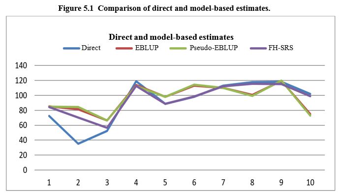
Description of Figure 5.1
Figure comparing the area level direct estimates with the model-based unit level (EBLUP and pseudo-EBLUP) and area level estimates (FH-SRS). There are four lines on this graph. The lines for EBLUP and pseudo-EBLUP estimates are almost identical. The line for the FH-SRS estimates and the line for the direct estimates are quite similar in this example.
Figure 5.2 compares the standard errors of the direct and model-based estimators. The standard errors of the model-based estimators are the squared root of the estimated MSE. Both the unit level estimators EBLUP and pseudo-EBLUP have small and stable standard errors. As expected, pseudo-EBLUP has slightly larger standard errors than EBLUP. It is clear that the direct and FH-SRS standard errors are very variable and are very unstable. This example shows the effectiveness of the unit level EBLUP and pseudo-EBLUP estimators.
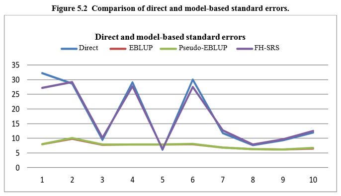
Description of Figure 5.2
Figure comparing the standard errors of the direct and model-based estimators. There are four lines on the graph. The standard errors of the model-based estimators are the squared root of the estimated MSE. Both the unit level estimators EBLUP and pseudo-EBLUP lines show small and stable standard errors. The pseudo-EBLUP line is slightly higher than EBLUP line. Lines associated with the direct and FH-SRS standard errors are very variable, very unstable and almost always higher than the EBLUP and pseudo-EBLUP lines.
- Date modified: