4 Study of the mean electricity consumption curve

Hervé Cardot, Alain Dessertaine, Camelia Goga, Étienne Josserand and Pauline Lardin

Previous | Next

We have a population $U$ consisting of $N=15,069$ electricity consumption curves measured every half hour during two consecutive weeks. We have $D=336$ measurement points for each week, and we want to estimate the mean consumption curve for the second week. We denote by $Y{\prime }_k=\left(Y_k\left(t_1\right)\mathrm{,}\dots \mathrm{,}{Y}_k\left(t_D\right)\right)\mathrm{,}$ the electricity consumption of individual $k\in U$ measured in the second week and $X{\prime }_k=\left(X_k\left(t_1\right)\mathrm{,}\dots \mathrm{,}{X}_k\left(t_D\right)\right)$, the individual's consumption during the first week. The mean consumption of each individual $k$ during the first week, $x_k={\displaystyle {\sum }_{d=1}^D{X}_k\left(t_d\right)/D}$, which is simple piece of information that is inexpensive to transmit, will be used as auxiliary information. 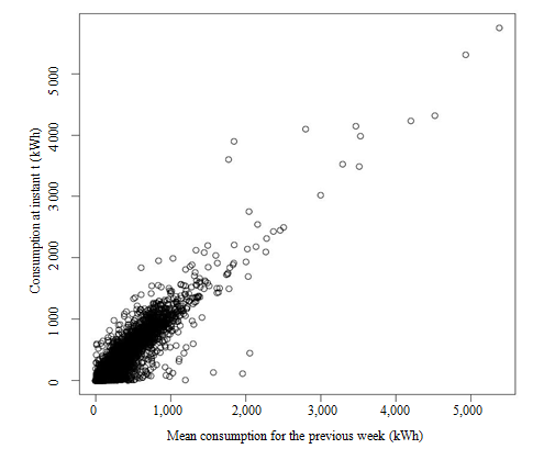This variable (a real one), which is known for all units $k$ in the population, is strongly related to the current consumption curve. As Figure 4.1 shows, the current consumption in each $t$ is almost proportional to the mean consumption for the previous week.

Description for figure 4.1

Figure 4.1 Representation of consumption at an instant $t$ as a function of the mean consumption for the previous week.

4.1 Description of strategies used

We consider samples of fixed size $n=1,500$ obtained using different sampling designs. The strategies presented are repeated $I$ times to evaluate and compare their performance.

1. SRSWOR sampling and Horvitz-Thompson estimator

This design is simple to implement; the Horvitz-Thompson estimator of the mean curve is given by (2.6) and the estimator of its covariance by (2.7).

2.STRAT stratified design and Horvitz-Thompson estimator

A stratified design is very effective if the strata are homogenous in relation to the variable of interest. In this study, we used the $k­$ means algorithm to create the strata, and we considered $H=10$ strata. A first stratification (STRAT 1) was carried out using the classification of the discretized trajectories ${X^{\prime }}_k$ for the previous week. A second stratification, which uses only the aggregate information $x_k$ was also considered. It is denoted by STRAT 2.

Tables 4.1 and 4.2 show the sizes of the strata $N_h$ yielded using the two stratifications and the optimal sizes $n_h$, according to (2.5), of the samples to be selected in each stratum. In both cases, the strata are numbered in ascending order in relation to the mean consumption for each stratum. More specifically, stratum 1 corresponds to small consumers of electricity and stratum 10 refers to the 10 largest consumers. Note that the first stratification, which requires knowing the electricity consumption at each measurement instant $t,$ requires more information than the second stratification. The mean curve is constructed using (2.3), and its covariance is estimated by (2.4).

 

Table 4.1
STRAT 1: stratification based on curves. The strata are constructed using the curves for week 1. The optimal allocation $n_h$ is calculated using the curves for week 1.
Table summary
This table displays stratification based on curves. The information is grouped by h (appearing as row headers), 1, 2, 3, 4, 5, 6, 7, 8, 9, 10 (appearing as column headers).

h	1	2	3	4	5	6	7	8	9	10
N h	3,866	4,769	623	2,690	664	1,251	806	328	62	10
n h	212	345	87	242	117	179	172	101	35	10

 

Table 4.2
STRAT 2: stratification based on the mean consumption $x_k.$ The optimal allocation $n_h$ is calculated using the mean consumption for week 1.
Table summary
This table displays stratification based on the mean consumption $x_k.$ The information is grouped by h (appearing as row headers), 1, 2, 3, 4, 5, 6, 7, 8, 9, 10 (appearing as column headers).

h	1	2	3	4	5	6	7	8	9	10
N h	3,257	4,236	3,139	1,937	1,189	731	415	125	30	10
n h	260	293	248	204	159	133	111	56	26	10

3. $\pi ps$ sampling and Horvitz-Thompson estimator

We used the cube algorithm proposed by Deville and Tillé (2004) and Chauvet and Tillé (2006), where the inclusion probabilities are proportional to $x_k\mathrm{,}k\in U$. To have a sampling design close to maximum entropy, a random sort of the population is performed before selection of the sample $s\mathrm{.}$ The covariance of the estimator of the mean is estimated using Formula (2.9). The cube algorithm is available in R in the sampling package, samplecube function, and a SAS macro is available on the INSEE website (Institut National de Statistique et des Études Économiques).

4. SRSWOR sampling and MA estimator

The estimator ${\widehat{\mu }}_{MA}$ assisted by the model $\xi$ is constructed using the auxiliary information given by $x{\prime }_k=\left(\mathrm{1,}{x}_k\right)$, where $x_k$ is the mean consumption for the previous week. In these conditions, ${\widehat{\mu }}_{MA}$ is the sum over any population $U$ of the values ${\widehat{Y}}_k$ estimated by the model (cf. Formula (2.13)). The covariance of the estimator of the mean is estimated using Formula (2.15).

4.2  Error of estimation of the mean curve

The error of estimation of the mean curve $\mu$ at instants $t_1\mathrm{,...,}{t}_{336}\mathrm{,}$ is evaluated according to the following criterion:

$R_2\left(\widehat{\mu }\right)=\frac{1}{336}{\displaystyle \sum _{i=1}^{336}}{\left(\widehat{\mu }\left(t_i\right)-\mu \left(t_i\right)\right)}^2\approx \frac{1}{T}{\displaystyle {\int }_0^T}{\left(\widehat{\mu }\left(t\right)-\mu \left(t\right)\right)}^{2}dt\mathrm{.}$

The results are shown in Table 4.3 for $I=10,000$ simulations (replications). They clearly show that for this study, taking account of total consumption for the previous week substantially improves the precision of the estimate of the mean compared with simple random sampling without replacement, dividing the mean square error $R_2$ by 5. Among the different strategies, the best appear to be those that take account of auxiliary information via inclusion probabilities (STRAT, $\pi ps$ and systematic PPS).

Table 4.3
Square error $R_2$ of estimation of the mean $\mu ,$ with $I=10,000$ replications
Table summary
This table displays square error $R_2$ of estimation of the mean $\mu ,$ with $I=10,000$ replications. The information is grouped by strategy (appearing as row headers), mean, 1^st, median, 3^rd (appearing as column headers).

Strategy	Mean	1 st quartile	Median	3 rdquartile
SRSWOR	40.53	10.82	22.16	51.09
STRAT (1)	5.78	3.68	5.08	7.07
STRAT (2)	6.49	4.03	5.48	7.88
$\pi ps$	7.06	3.99	5.52	8.16
Systematic  $\pi -ps$	6.73	3.85	5.20	8.07
MA	8.29	5.24	7.14	10.16

4.3  Coverage rate and width of confidence bands

The construction of confidence bands of level $1-\alpha$ requires calculating quantiles of order $1-\alpha$ of the supremum of Gaussian processes.

So as not to favour one method of constructing confidence bands over the other, we applied the two algorithms to the same sample $s$ and we considered the same number $M$ of processes. This number $M$ varies from one estimator to the other owing to the computation time needed for the bootstrap approaches (see Section 4.4).

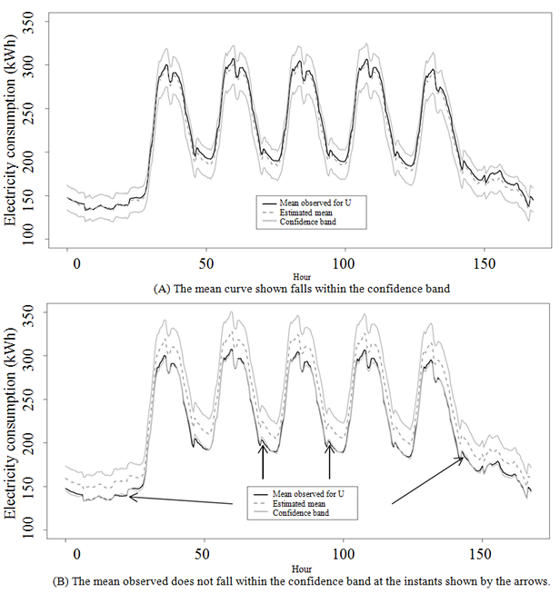
Description for figure 4.2

Figure 4.2 Examples of confidence bands.

The empirical coverage rate is the proportion of times, among the $I=2,000$ replications, where the true mean curve $\mu$ appears, for all instants $t\mathrm{,}$ within the confidence band constructed using an estimate $\widehat{\mu }\mathrm{.}$ Figure 4.2 shows two examples of confidence bands (continuous grey curves) constructed from estimated curves (dotted grey curves). Figure 4.2(A) shows that the true mean curve for the population (continuous black curve) is within the confidence band at every instant. Conversely, Figure 4.2(B) shows that mean curve for the population is generally overestimated and there are a few instants (indicated by arrows) where the curve shown is outside the confidence band. Empirical coverage rates are shown in Table 4.4.

The two methods of constructing confidence bands yield coverage rates that are similar and fairly close to the desired nominal rates (95% and 99%). However, the results seem slightly less satisfactory for the $\pi ps$ designs and for the MA approach, for which the variance of the estimator is complex and more difficult to estimate precisely.

Table 4.4
Empirical coverage rate (in %), for $I=2,000$ replications
Table summary
This table displays empirical coverage rate (in %), for $I=2,000$ replications. The information is grouped by method (appearing as row headers), Number M of processes, Bootstrap, Gaussian process (appearing as column headers).

Method	Number M of processes	Bootstrap		Gaussian process
		$\alpha =0.05$	$\alpha =0.01$	$\alpha =0.05$	$\alpha =0.01$
SRSWOR	5,000	94.95	98.85	94.80	98.70
STRAT (1)	5,000	93.92	98.34	94.09	98.43
STRAT (2)	5,000	94.3	98.45	94	98.55
$\pi ps$	1,000	94.73	98.77	93.87	98.61
MA	5,000	94.3	98.5	92.85	98.15

Another useful indicator is the mean width of the confidence band,

$$\frac{1}{336}{\displaystyle \sum _{i=1}^{336}2c_{\alpha }\widehat{\sigma }\left(t_i\right)}\approx \frac{1}{T}{\displaystyle {\int }_0^T}2c_{\alpha }\widehat{\sigma }\left(t\right)dt$$

the values of which are shown in Table 4.5. The two methods provide confidence bands of largely similar width. Also note that the use of the auxiliary variable considerably reduces the mean band width, which is cut in half if one of the stratified designs is used rather than a SRSWOR design.

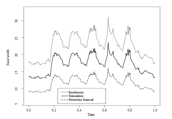
Description for figure 4.3

Figure 4.3 Simple random sampling without replacement. Width of confidence bands - pointwise, overall by process simulations, and with Bonferroni ( $\alpha =\text{0}\text{.05}$).

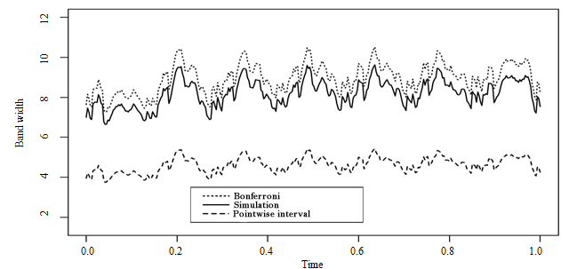
Description for figure 4.4

Figure 4.4 Stratified sampling (STRAT 1). Width of confidence bands - pointwise, overall by process simulations, and with Bonferroni (with $\alpha =\text{0}\text{.05}$).

Figures 4.3 and 4.4 show the widths of the confidence bands for a level $\alpha =0.05$ , for each instant, depending on whether they are pointwise ( $c_{\alpha }=1.96$), estimated by simulations of Gaussian processes or obtained using the approach based on the Bonferroni inequality applied to each measurement point. We then have, in the latter case, $c_{\alpha }=3.793048$, the quantile of order $1-\text{0}\text{.05}/\left(336\times 2\right)$ of a distribution $N\left(\mathrm{0,1}\right)\mathrm{.}$  The bands obtained by Bonferroni are conservative, and they cover what might be considered the worst case in terms of information, the case of independence of the pointwise intervals. Note that the simulation approach substantially reduces the mean width of the bands in comparison with Bonferroni when the design does not allow all temporal information on the data to be taken into account (Figure 4.3). Conversely, for the stratified design (Figure 4.4), which provides a precise estimate of the mean curve, the confidence band constructed by simulation is close to that of Bonferroni, which can intuitively be interpreted as meaning that almost all the information was captured by the sampling design.

Table 4.5
Mean width of confidence bands, for $I=2,000$ replications
Table summary
This table displays mean width of confidence bands, for $I=2,000$ replications. The information is grouped by method (appearing as row headers), number M of processes, bootstrap, gaussian process (appearing as column headers).

Method	Number M of processes	Bootstrap		Gaussian process
		$\alpha =0.05$	$\alpha =0.01$	$\alpha =0.05$	$\alpha =0.01$
SRSWOR	5,000	35.98	43.35	35.99	43.19
STRAT (1)	5,000	16.64	18.92	16.62	18.88
STRAT (2)	5,000	17.58	19.99	17.55	19.94
$\pi ps$	1,000	17.85	20.31	17.62	19.93
MA	5,000	19.88	22.65	19.75	22.44

4.4  Computation time

Computation times with the bootstrap method are much greater$—$by a factor of approximately 1 to 1,000$—$than those with the Gaussian processes simulation method (cf. Table 4.6). The reason for this major difference is that in the bootstrap methods, the entire estimation process (construction of the fictitious population, drawing of a new sample, calculation of the estimator) must be repeated for each bootstrapped sample. Also, the designs that introduce auxiliary information are slower than SRSWOR, even though if used individually their computation time is entirely reasonable.

Table 4.6
Run time of a simulation in seconds for $M=5,000$ replications. The SRSWOR, MA and STRAT strategies were programmed with R and $\pi ps$ with SAS.
Table summary
This table displays run time of a simulation in seconds for $M=5,000$ replications. The SRSWOR, MA and STRAT strategies were programmed with R and $\pi ps$ with SAS. The information is grouped by Strategy (appearing as row headers), bootstrap, Gaussian processes (appearing as column headers).

Strategy	Bootstrap	Gaussian processes
SRSWOR	1,170.6	1.0
STRAT	1,839.5	1.4
$\pi ps$	5,020.0	7.3
MA	3,156	1.4

Previous | Next