5. Results

Natalja Menold

Previous | Next

5.1 Differences between household types

Firstly, the results for testing hypothesis H1 are presented. This hypothesis expects deviations from the 50/50 gender ratio to vary according to the type of household. Figure 5.1 shows the differences $\left(d\right)$between the actual percentage of males and the expected true value of 50% in three subsamples. A 95% confidence interval (CI) was used to control for random fluctuation. As the expected proportion of men is $p=$0.5, the variance averages $0.25/n,$ whereby $n$ is the number of cases in the subsample in a country. The 95% CI was calculated as follows (cf. Kohler 2007, page 59):

$$CI=0.5\pm 1.96\times \sqrt{0.25/2}.$$

Figure 5.1 shows that for both subsamples covering households with children, significant values of $d$ are negative in the majority of cases, meaning that the proportion of males in these subsamples is less than 50% (as expected by H1). Most of these $d$-values were approx. 10% or higher. Lower (approx. 5%) significant positive (unexpected) $d$-values are seen for three countries in which PRS was used (in the ESS1 in Belgium and Norway, in the ESS2 in Finland). However, these differences were not discernible in other rounds.

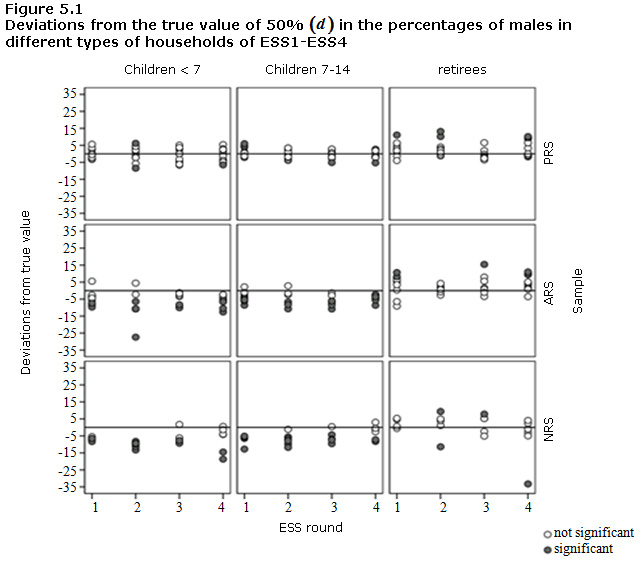
Description for figure 5.1

Regarding the results for the subsamples covering households with partners of retirement age (retirees) it is possible to see significantly high $d$-values (approx. 10% or higher) with the expected direction (positive, or that is to say the percentages of males are higher than 50%) for some countries across all sampling methods (in the ESS1 in Norway, the Czech Republic and the Netherlands; in the ESS 2 in Norway, Poland and France; in the ESS3 in Cyprus and Russia and in the ESS4 in Germany, Hungary, Cyprus and the United Kingdom). Interestingly, the proportion of men is markedly lower than 50% in Slovakia in the ESS4 (as low as approx. 33%) and in Portugal in the ESS2 (as low as approx. 11%). This result can be explained by specific patterns of role division between the partners. Here the woman appears to represent the household, even if the man is at home.

To summarise, significant deviations from true value in different types of households were mainly in line with the expectations of hypothesis H1.

5.2 Differences between sampling methods

The effect of sampling methods (as expected by H2) was tested by means of MANCOVA. The $d$-values for the three types of households (three isolated subsamples) were considered as values of three dependent variables, which were simultaneously analysed in the MANCOVA. Since the MANCOVA is based on an analysis of means the absolute values of $d$ were considered. Otherwise it would not have been possible to take into account differences with an unexpected direction, which would also be associated with the effect of sampling methods. Since most of the differences were negative in the subsamples with children, the absolute $d$-values represent a proportion of men that is lower than 50%. With respect to the subsamples with partners of retirement age, it should be taken into account that the proportion of men was not only higher than 50% but also lower than 50% in Portugal (ESS2) and in Slovakia (ESS4). In addition, significant and non-significant differences are considered in order to enable a comparison between countries with low and high $d$-values.

The MANCOVA revealed a high significant multivariate effect of the factor "sampling method" (Wilks Lambda (WL) $F_{\left(6,174\right)}=6.87,p<0.001,$ effect size ${\eta }^2=0.21$ ). In contrast, no significant results for explanatory variables were found ( $p>0.10,$ max ${\eta }^2=0.04$ ). In order to consider $d$-values in different household types univariate analyses of covariance (ANCOVAs) were employed. Variance homogeneity $–$ as a presupposition for an ANCOVA $–$ is given according to the Levene test in the subsample with retirees, and also according to the $F_{\max }$ test in the subsamples with children. Significant mean differences of $d$-values between sampling methods were found using the ANCOVAs in both subsamples with children (table 5.1). The variances explained in the ANCOVAs for these subsamples are quite high (see $R^2$ in table 5.1). On average the lowest $d$-value can be seen for the PRS, while the highest $d$-value is seen for the NRS (table 5.1 and figure 5.2). However, post-hoc single comparisons using subsamples with children show significant differences only between PRS and the other two sampling methods (table 5.2). Also, no remarkable differences in $d$-values were found between the countries with ALS and with Random Route samples.

Overall, the results show that hypothesis H2 can be partially supported if households with children are considered.

Table 5.1
Descriptive statistics $\left(M\left(SD\right)\right)$ and results of the ANCOVAs for comparison of $d$ in the three types of household
Table summary
This table displays the results of Descriptive statistics $\left(M\left(SD\right)\right)$ and results of the ANCOVAs for comparison of $d$ in the three types of household types of household (appearing as column headers).

	types of household
	children <7	children 7-14	retirees	$n$ (countries)
Sampling method (treatment)
PRS	3.28(2.07)	2.21(1.37)	3.34 (3.35)	43
ARS	6.61(4.98)	4.87 (2.74)	4.94(3.83)	31
NRS	7.85 (4.4)	5.92 (3.55)	5.78(6.87)	21
$F\left(d{f}_1=1,d{f}_2=88\right)$	14.52***	20.9***	1.93
Time: ESS round
1	4.49(2.67)	4.08(2.94)	4.75(3.22)	22
2	6.92(5.73)	4.33(3.3)	3.63(3.71)	24
3	4.78(3.04)	4.02(3.18)	3.74(3.44)	23
4	5.23(4.41)	3.24(2.22)	5.39(6.66)	26
$F\left(d{f}_1=1,d{f}_2=88\right)$	0	1.18	0.02
Payment bonus
no	5.83(4.37)	4.41(3.10)	4.10(3.73)	54
yes	4.78(3.99)	3.23(2.52)	4.81(5.49)	41
$F\left(d{f}_1=1,d{f}_2=88\right)$	0.57	3.21+	0.49
Ratio controlled
$F\left(d{f}_1=1,d{f}_2=88\right)$	0.11	0.51	1.09
Ratio confirmed
$F\left(d{f}_1=1,d{f}_2=88\right)$	3.11+	0.11	0
$R^2$	0.22	0.31	0.01
Notes ***$p<0.001$, +$p<0.10$.

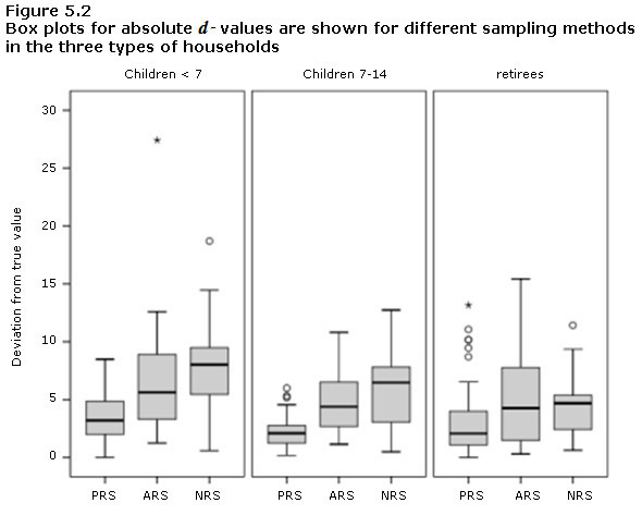
Description for figure 5.2

Table 5.2
Mean differences of $\left(d\left(SD\right)\right)$ between sampling methods in subsamples with children
Table summary
This table displays the results of Mean differences of $\left(d\left(SD\right)\right)$ between sampling methods in subsamples with children children <7 and children 7-14 (appearing as column headers).

	children <7	children 7-14
differences between
PRS and ARS	-3.34 (0.89)**	-2.66 (0.58)**
PRS and NRS	-4.58 (1.0)**	-3.71 (0.65)**
ARS and NRS	-1.24 (1.07)	-1.05 (0.7)

Note **$p<0.01$ Single post hoc tests with Bonferroni correction.

5.3 The effect of explanatory variables

The effect of explanatory variables was analysed to test hypothesis H3, which expects deviations from the 50/50 gender ratio to be stable across time and to correlate with payment, interviewer controls and change of data collector.

Some countries in the ESS changed their sampling method procedures and/or data collector between the rounds (see appendix). The results showed that neither multivariate effects $\left(\text{WL}{F}_{\left(3,85\right)}=0.81,p>0.10\right)$nor univariate effects are significant for the change of data collector. Thus, table 5.1 presents the ANCOVA results without this variable. If the "change of data collector" is included in the analyses, then the effect of the variable "ratio confirmed" is no longer significant, but this does not impact the effects of any of the other variables. This result shows that a change of data collectors may correlate with control procedures. The differences in $d$-values across the ESS rounds are not significant either, neither within multivariate analysis $\left(\text{WL}{F}_{\left(3,86\right)}=0.51,p>0.10\right)$nor within the univariate analyses (for the latter see table 5.1).

Table 5.1 shows that in subsamples with children $d$-value means are lower if a payment bonus is used as compared to when it is not used. However, this difference is significant only on a 10% level $\left(p<0.10\right)$and only in households with older children. Hence, this result shows that payment methods may play a role, thereby reducing deviation from the true value in the case of higher payments.

Regarding control procedures, the number of controls ("ratio selected") is not related to the value of $d$ (table 5.1). The success rate in controls ("ratio confirmed") is related to the value of $d$ in the subsample with children younger than seven years old. This relationship is negative $\left(B=-0.06;SE=0.04\right),$meaning that the lower the confirmed control rates are, the higher the values of $d$ are. However, this relationship is also significant only at a 10% level.

Concerning hypothesis H3, it has been shown that the effect of sampling methods is independent of the time effect. The results support the expectation of H3 concerning interviewer payment and controls. However, the results for these variables show that these effects are only weak and they can only be found in some household types.

Previous | Next