4. Simulation study

John Preston

Previous | Next

A Monte Carlo simulation study was conducted to examine the performance of the proposed composite regression estimator. Ten artificial populations were created for the simulation study. Firstly, a base population (Population I) was generated to resemble the physical appearance of typical monthly business surveys conducted over a five year time period. Secondly, six additional populations (Populations II to VII) were each generated by modifying one of six key characteristics of the base population to help determine whether this particular characteristic had an impact on the performance of the proposed composite regression estimator. Finally, three supplementary populations (Populations VIII to X) were generated to examine the impact of auxiliary variables on the performance of the proposed composite regression estimator. A brief description of the ten artificial populations is given in Table 4.1.

The population totals at time $t$ for the various artificial populations were produced using the time series model:

$$Y^{\left(t\right)}=T^{\left(t\right)}+{\alpha }_2{S}^{\left(t\right)}+{\alpha }_3{I}^{\left(t\right)}$$

where $T^{\left(t\right)},S^{\left(t\right)}$ and $I^{\left(t\right)}$ are the trend, seasonality and irregular components of the time series given by:

$$T^{\left(t\right)}=\text{1,000}+5\left(t-1\right)+50\left(1-\cos \left(\pi \left(t-1\right)/18\right)\right)$$

$$S^{\left(t\right)}=25\left[\sin \left(\pi t/6\right)-\cos \left(\pi t/6\right)+\cos \left(\pi t/3\right)\right]$$

$$I^{\left(t\right)}=25{\epsilon }^{\left(t\right)}$$

with ${\alpha }_2=1$ for all artificial populations, except Population II (high seasonal series) where ${\alpha }_2=4,$ and ${\alpha }_3=1$ for all artificial populations, except Population III (high irregular series) where ${\alpha }_3=4,$ and ${\epsilon }^{\left(t\right)}\sim N\left(0,1\right).$ The original $\left(T^{\left(t\right)}+S^{\left(t\right)}+I^{\left(t\right)}\right),$ seasonally adjusted $\left(T^{\left(t\right)}+I^{\left(t\right)}\right)$ and trend $\left(T^{\left(t\right)}\right)$ series for the base artificial population are presented in Figure 4.1.

Table 4.1
Description of the artificial populations
Table summary
This table displays the results of Description of the artificial populations. The information is grouped by Artificial Populations (appearing as row headers), Population Descriptions (appearing as column headers).

Artificial Populations	Population Descriptions
Population I	Base Series
Population II	High Seasonal Series
Population III	High Irregular Series
Population IV	High Population Rotation Series
Population V	High Sample Rotation Series
Population VI	High Unit Variation Series
Population VII	Low Unit Correlation Series
Population VIII	Base Auxiliary Correlation Series
Population IX	High Auxiliary Correlation Series
Population X	Low Auxiliary Correlation Series

Figure 4.1 Time series for population I

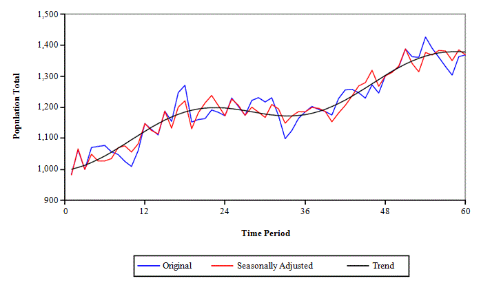
Description for Figure 4.1

All ten artificial populations were partitioned into five strata; four take-some strata $\left(h=1,\dots ,4\right)$ and one take-all strata $\left(h=5\right).$ The stratum population sizes at time $t$ were chosen as $N_h^{\left(t\right)}=N_h\left[1+0.5\left(T^{\left(t\right)}/T^{\left(1\right)}-1\right)\right],$ where $N_h$ is the stratum population for all artificial populations at time 1, selected to yield a skewed population often associated with typical business.

The expected population rotation rates between time $t-1$ and time $t,$ due to the addition of "births� and the deletion of "deaths�, were specified as ${\alpha }_4\left(1-R_h\right),$ where $R_h$ is the probability of a unit being "deathed� in the population for the base artificial population at any time period. A value of ${\alpha }_4=1$ was used for all artificial populations, except Population IV (high population rotation series) where ${\alpha }_4=2$ was used. The stratum sample sizes at time $t$ were set to $n_h^{\left(t\right)}=n_h$ for the take-some strata, and $n_h^{\left(t\right)}=N_h^{\left(t\right)}$ for the take-all strata, where $n_h$ is the stratum population at time 1.

The planned sample rotation rates between time $t-1$ and time $t$ were specified as ${\alpha }_5\left(1-r_h\right),$ where $r_h$ is equal to the inverse of the number of consecutive survey cycles a unit is expected to be in the sample given no population rotation, for the base artificial population at any time period (e.g., a planned sample rotation rate of 0.0417 equates to 24 survey cycles). A value of ${\alpha }_5=1$ was used for all artificial populations, except Population V (high sample rotation series) where ${\alpha }_5=2$ was used. The actual sample rotation rates will depend on these planned sample rotation as well as any unplanned sample rotation caused by the population rotation. The expected population rotation rates and the planned stratum sample rotation rate were selected to yield population and sample rotation rates similar to those often encountered in typical business surveys.

The stratum averages and stratum population variances at time $t$ were specified respectively as ${\overline{y}}_h^{\left(t\right)}=0.2\left(Y^{\left(t\right)}/N_h^{\left(t\right)}\right)$ and $S_h^{\left(t\right)2}={\alpha }_6{S}_h^2{\left({\overline{y}}_h^{\left(t\right)}/{\overline{y}}_h^{\left(t\right)}\right)}^2$ with ${\alpha }_6=1$ for all artificial populations, except Population VI (high unit variation series) where ${\alpha }_6=4.$ The stratum population correlations between time $t$ and time $t-k$ were defined using an exponential decay model, $\rho \left(y_h^{\left(t\right)},y_h^{\left(t-k\right)}\right)=\exp \left(-0.02{\alpha }_{7}k\right)$ with ${\alpha }_7=1$ for all artificial populations, except Population VII (low unit correlation series) where ${\alpha }_7=4.$ The stratum population correlations between the variable of interest and the auxiliary variable at time $t$ were defined as $\rho \left(x_h^{\left(t\right)},y_h^{\left(t\right)}\right)=1-{\alpha }_8\left(1-{\rho }_h\right)$ with ${\alpha }_8=1$ for Population VIII (base auxiliary correlation series), ${\alpha }_8=0.5$ for Population IX (high auxiliary correlation series), ${\alpha }_8=1.5$ for Population X (low auxiliary correlation series) and not applicable for all other artificial populations.

The variables of interest $y_{hi}^{\left(t\right)}$ and auxiliary variables $x_{hi}^{\left(t\right)}$ for unit $i$ in stratum $h$ at time $t$ were generated from multivariate lognormal distributions with means ${\overline{y}}_h^{\left(t\right)},$ variances $S_h^{\left(t\right)2}$ and correlation coefficients $\rho \left(y_h^{\left(t\right)},y_h^{\left(t-k\right)}\right).$ The stratum level characteristics of $N_h,n_h,R_h,r_h$ and $S_h^2$ are given by the values presented in Table 4.2.

A total of $S=\text{10,000}$ independent simulations were conducted for each of the ten artificial populations. In each of these simulations, stratified random samples $s_h^{\left(t\right)}$ of size $n_h^{\left(t\right)}$ were selected from the population $U_h^{\left(t\right)}$ using a permanent random number (PRN) selection technique at each time period, $t=1,\dots ,60.$ At each time period, $t>1,$ the "pseudo-populations�, $U_h^{*\left(t-1\right)}$ and $U_h^{*\left(t\right)},$ and "pseudo-samples�, $s_h^{*\left(t-1\right)}$ and $s_h^{*\left(t\right)},$ were identified, and the various MR estimators were evaluated. These included the MR1 estimator $\left(\alpha =0\right);$ the MR2 estimator $\left(\alpha =1\right);$ the MR estimator using $\alpha =\text{0}\text{.25},\text{0}\text{.5}$ and $0.75\text{;}$ the MRR estimator and the MRC estimator, with a compromise between the HT estimator and the MRR estimator for Populations I to VII and the GR estimator and the MRR estimator for Populations VIII to $X,$ using $\alpha =0.25,0.5$ and $\mathrm{0.75.}$

Table 4.2
Stratum characteristics
Table summary
This table displays the results of Stratum characteristics. The information is grouped by XXXX (appearing as row headers), XXXX (appearing as column headers).

$h$	$N_h$	$R_h$	$n_h$	$r_h$	$S_h^2$	${\rho }_h$
S1	8,000	0.0150	12	0.042	0.4	0.85
S2	1,600	0.0125	18	0.042	3	0.75
S3	320	0.0100	24	0.042	20	0.65
S4	64	0.0075	30	0.000	125	0.55
S5	16	0.0025	16	0.000	625	0.95

The performance of the various MR estimators for the point-in-time and movement estimates were compared using their relative biases and the relative efficiencies with respect to the HT estimator for all artificial populations and also with respect to the GR estimator for Populations VIII to X. The relative biases and relative efficiencies of variable of interest $y$ at time $t$ for the point-in-time and movement estimates were calculated as:

$$\begin{array}{lll}\text{RB}\left({\widehat{Y}}^{\left(t\right)}\right)\hfill & =\hfill & \frac{1}{Y^{\left(t\right)}}\left[\frac{1}{S}{\displaystyle \sum _{s=1}^S\left({\widehat{Y}}_s^{\left(t\right)}-Y^{\left(t\right)}\right)}\right]\hfill \\ \text{RB}\left({\widehat{Y}}^{\left(t\right)}-{\widehat{Y}}^{\left(t-1\right)}\right)\hfill & =\hfill & \frac{1}{Y^{\left(t-1\right)}}\left[\frac{1}{S}{\displaystyle \sum _{s=1}^S\left(\left({\widehat{Y}}_s^{\left(t\right)}-{\widehat{Y}}_s^{\left(t-1\right)}\right)-\left(Y^{\left(t\right)}-Y^{\left(t-1\right)}\right)\right)}\right]\hfill \\ \text{RE}\left({\widehat{Y}}^{\left(t\right)}\right)\hfill & =\hfill & \text{MSE}\left({\widehat{Y}}_{*}^{\left(t\right)}\right)/\text{MSE}\left({\widehat{Y}}^{\left(t\right)}\right)\hfill \\ \text{RE}\left({\widehat{Y}}^{\left(t\right)}-{\widehat{Y}}^{\left(t-1\right)}\right)\hfill & =\hfill & \text{MSE}\left({\widehat{Y}}_{*}^{\left(t\right)}-{\widehat{Y}}_{*}^{\left(t-1\right)}\right)/\text{MSE}\left({\widehat{Y}}^{\left(t\right)}-{\widehat{Y}}^{\left(t-1\right)}\right)\hfill \end{array}$$

where ${\widehat{Y}}_s^{\left(t\right)}$ is the estimator for variable of interest $y$ at time $t$ for the $s^{\text{th}}$ simulation sample, ${\widehat{Y}}_{*}^{\left(t\right)}$ is the HT or GR estimator for variable of interest $y$ at time $t,$ and $\text{MSE}\left({\widehat{Y}}^{\left(t\right)}\right)$ and $\text{MSE}\left({\widehat{Y}}^{\left(t\right)}-{\widehat{Y}}^{\left(t-1\right)}\right)$ are the mean squared errors for variable of interest $y$ at time $t$ for the point-in-time and movement estimates given by:

$$\begin{array}{lll}\text{MSE}\left({\widehat{Y}}^{\left(t\right)}\right)\hfill & =\hfill & \frac{1}{S}{\displaystyle \sum _{s=1}^S{\left({\widehat{Y}}_s^{\left(t\right)}-Y^{\left(t\right)}\right)}^2}\hfill \\ \text{MSE}\left({\widehat{Y}}^{\left(t\right)}-{\widehat{Y}}^{\left(t-1\right)}\right)\hfill & =\hfill & \frac{1}{S}{\displaystyle \sum _{s=1}^S{\left(\left({\widehat{Y}}_s^{\left(t\right)}-{\widehat{Y}}_s^{\left(t-1\right)}\right)-\left(Y^{\left(t\right)}-Y^{\left(t-1\right)}\right)\right)}^2}.\hfill \end{array}$$

The relative biases of the point-in-time estimates for the MR1, MR2 and MRR estimators, averaged over the twelve months within each of the five years, for Population I (base series) are shown in Table 4.3. The proposed MR estimators (MR1-P, MR2-P, MRR-P) were compared against the current MR estimators (MR1-C, MR2-C, MRR-C), and the adjusted MR estimators (MR1-A, MR2-A, MRR-A), where a correction factor was applied to the MR values to account for the relative change in the population size in stratum $h$ between time $t-1$ and time $t.$

Table 4.3
Average relative bias (%) of point-in-time estimates for population I
Table summary
This table displays the results of Average relative bias (%) of point-in-time estimates for population I Year 1, Year 2, Year 3, Year 4 and Year 5 (appearing as column headers).

	Year 1	Year 2	Year 3	Year 4	Year 5
HT	0.024	-0.032	-0.015	-0.003	-0.005
MR1-C	-0.909	-2.871	-2.292	-2.836	-4.122
MR2-C	-0.918	-3.432	-3.449	-4.502	-6.820
MRR-C	-0.919	-3.437	-3.458	-4.515	-6.839
MR1-A	0.064	-0.129	0.002	-0.062	-0.068
MR2-A	0.169	0.024	0.039	-0.109	-0.317
MRR-A	0.152	-0.027	-0.014	-0.174	-0.410
MR1-P	0.009	-0.066	-0.040	-0.051	-0.054
MR2-P	0.022	-0.053	-0.028	-0.039	-0.034
MRR-P	0.020	-0.056	-0.030	-0.039	-0.036

The current MR estimators exhibit substantial negative biases which compound over time. While the adjusted MR estimator removes the majority of these biases, the MR2-A and MRR-A estimators still display small negative biases which compound over time. On the other hand, the relative biases of the proposed MR estimator are negligible, with no apparent change in the magnitude of the relative biases over the five years.

Table 4.4 presents the absolute relative biases and relative efficiencies of the estimators for Population I (base series), averaged over the twelve months within each of the five years. The average absolute relative biases of the point-in-time and movement estimates were negligible for all of the estimators, and there was no appreciable change in the magnitude of the relative biases in any of the estimators over the five years. For the point-in-time estimates, the MR1 estimator performed better than the HT estimator, while the MR2 and MRR estimators performed poorer than the HT estimator. The relative efficiency of the MR2 and MRR estimators declined substantially over the five years, which suggests that these estimators are susceptible to the "drift� problem. The presence of the "drift� problem is evident by observing the relationship between the point-in-time estimates at the start of the first year $\left(t=1\right)$ and those at the start of the third year $\left(t=25\right)$ from the simulation samples (Figure 4.2).

It can be seen that there are positive correlations between the point-in-time estimates at the start of the first and third years for the MR1, MR2, MRR and MR $\left(\alpha =0.75\right)$ estimators, signifying that once these estimators vary greatly from the true population totals, then there is a high likelihood that they will continue to drift further from the true population totals over time. While the correlations for the MR1 estimator are lower than those for the MR2 estimator, positive correlations are still evident signifying that the MR1 estimator is not immune from the drift problem. The positive correlations are not apparent for the HT and MRC $\left(\alpha =0.25\right)$ estimators, and hence these estimators are not prone to the "drift� problem. Furthermore, it is clear that the MR2, MRR and MR $\left(\alpha =0.75\right)$ estimators are much more variable than the HT, MR1 and MRC $\left(\alpha =0.25\right)$ estimators at start of the third year.

Table 4.4
Average absolute relative bias (%) and average relative efficiency (%) for population I
Table summary
This table displays the results of Average absolute relative bias (%) and average relative efficiency (%) for population I Point-in-Time Estimates, Movement Estimates, Year 1, Year 2, Year 3, Year 4 and Year 5 (appearing as column headers).

	Point-in-Time Estimates					Movement Estimates
	Year 1	Year 2	Year 3	Year 4	Year 5	Year 1	Year 2	Year 3	Year 4	Year 5
	Average Absolute Relative Bias (%)
$\text{HT}$	0.031	0.032	0.030	0.025	0.010	0.021	0.011	0.012	0.019	0.014
$\text{MR1}$	0.032	0.066	0.041	0.051	0.054	0.021	0.011	0.010	0.010	0.016
$\text{MR2}$	0.024	0.053	0.030	0.039	0.034	0.014	0.009	0.009	0.009	0.013
$\text{MR}\left(\alpha =0.25\right)$	0.029	0.067	0.045	0.058	0.063	0.019	0.010	0.009	0.009	0.015
$\text{MR}\left(\alpha =0.50\right)$	0.027	0.066	0.045	0.060	0.064	0.017	0.010	0.009	0.009	0.014
$\text{MR}\left(\alpha =0.75\right)$	0.025	0.061	0.040	0.054	0.055	0.016	0.009	0.009	0.009	0.014
$\text{MRR}$	0.023	0.056	0.032	0.040	0.036	0.014	0.009	0.009	0.009	0.013
$\text{MRC}\left(\alpha =0.25\right)$	0.027	0.041	0.025	0.018	0.011	0.016	0.009	0.010	0.009	0.014
$\text{MRC}\left(\alpha =0.50\right)$	0.028	0.036	0.028	0.021	0.010	0.018	0.008	0.011	0.010	0.014
$\text{MRC}\left(\alpha =0.75\right)$	0.029	0.033	0.029	0.024	0.010	0.019	0.008	0.011	0.014	0.014
	Average Relative Efficiency (%)
$\text{HT}$	100.0	100.0	100.0	100.0	100.0	100.0	100.0	100.0	100.0	100.0
$\text{MR1}$	122.0	126.0	118.4	112.7	114.6	137.6	132.8	132.7	134.2	133.0
$\text{MR2}$	92.4	74.7	57.7	47.8	45.8	223.0	203.0	206.5	206.4	204.8
$\text{MR}\left(\alpha =0.25\right)$	121.6	123.4	110.6	100.9	100.9	168.3	158.4	159.7	160.7	159.2
$\text{MR}\left(\alpha =0.50\right)$	115.3	110.0	92.8	80.9	79.3	199.0	182.8	185.6	186.0	184.3
$\text{MR}\left(\alpha =0.75\right)$	104.7	91.9	73.5	62.0	59.7	220.4	199.6	203.5	203.4	201.6
$\text{MRR}$	94.1	79.6	63.0	53.4	53.1	223.3	203.3	206.9	206.8	204.8
$\text{MRC}\left(\alpha =0.25\right)$	110.8	113.7	113.1	113.7	113.1	198.5	182.7	186.5	187.1	184.4
$\text{MRC}\left(\alpha =0.50\right)$	106.0	105.9	105.6	105.9	105.5	164.2	155.0	157.3	157.6	155.8
$\text{MRC}\left(\alpha =0.75\right)$	102.7	102.4	102.3	102.4	102.3	130.9	127.4	128.3	128.4	127.6

An appropriate choice of $\alpha$ for the MRC estimators will minimize the likelihood of the "drift� problem. Compared to the MRR estimator, this MRC $\left(\alpha =0.25\right)$ estimator will improve the efficiency of the point-in-time estimates, but reduce the efficiency of the movement estimates. For the movement estimates, the MR1 estimator performed slightly better than the HT estimator while the MR2 and MRR estimators performed considerably better than the HT estimator. Overall, the MRC estimator appears to perform slightly better than MR estimator. If the objective is to choose an estimator which is not too susceptible to the "drift� problem and which maximises the efficiency of the movement estimates without any loss in relative efficiency for the point-in-times estimates, then the "best� estimator for this particular population is the MRC estimator with $\alpha \approx \mathrm{0.10.}$ This estimator is likely to have minimal drift and leads to moderate efficiency gains of 21.6 percent in the point-in-time estimates and significant efficiency gains of 104.2 percent in the movement estimates.

The average absolute relative biases and average relative efficiencies of the estimators for Populations I to VII are shown in Table 4.5. Large increases in the seasonality (Population II) or irregularity (Population III) of the time series had almost no impact on the performance of the various estimators for the point-in-time estimates. While there were small reductions in the relative efficiency of the movement estimates for MR2 and MRR estimators, there was no impact for the MR1 estimator.

Figure 4.2 Plots of various estimators for population I

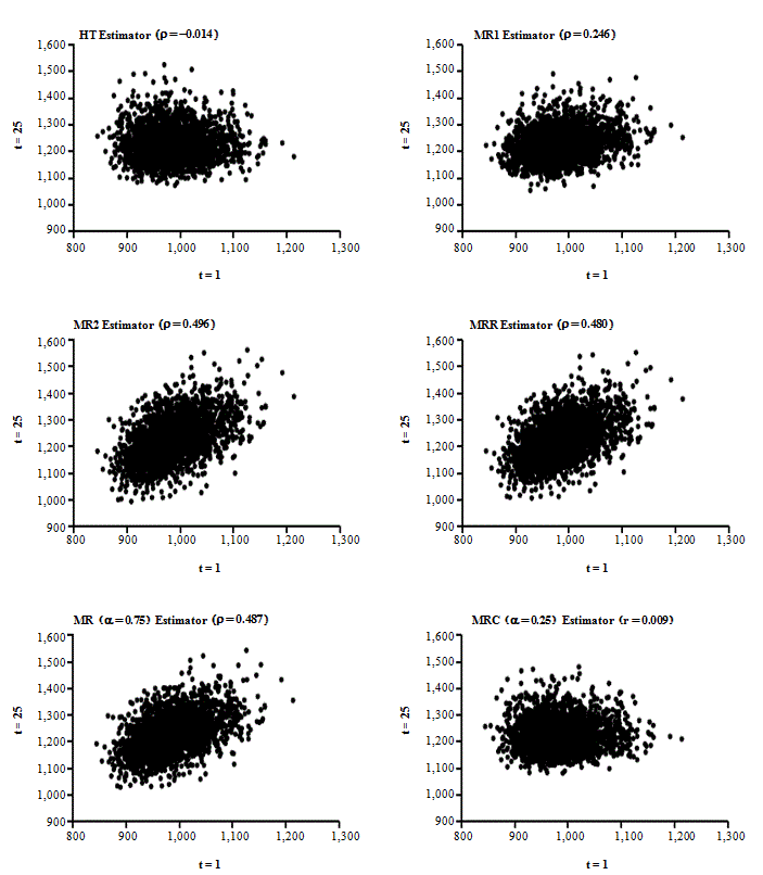
Description for Figure 4.2

Table 4.5
Average absolute relative bias (%) and average relative efficiency (%)
Table summary
This table displays the results of Average absolute relative bias (%) and average relative efficiency (%) Point-in-Time Estimates, Movement Estimates, Pop, I, II, III, IV, V, VI and VII (appearing as column headers).

	Point-in-Time Estimates							Movement Estimates
	Average Absolute Relative Bias (%)
$\text{HT}$	0.038	0.027	0.049	0.048	0.048	0.065	0.032	0.017	0.012	0.016	0.018	0.020	0.025	0.020
$\text{MR1}$	0.050	0.098	0.074	0.052	0.089	0.150	0.078	0.014	0.012	0.013	0.015	0.020	0.020	0.018
$\text{MR2}$	0.081	0.028	0.039	0.063	0.047	0.218	0.120	0.012	0.011	0.011	0.014	0.013	0.017	0.017
$\text{MR}\left(\alpha =0.25\right)$	0.052	0.083	0.070	0.046	0.095	0.139	0.090	0.013	0.011	0.012	0.014	0.018	0.018	0.017
$\text{MR}\left(\alpha =0.50\right)$	0.057	0.058	0.059	0.043	0.089	0.136	0.103	0.012	0.010	0.011	0.014	0.016	0.016	0.017
$\text{MR}\left(\alpha =0.75\right)$	0.066	0.038	0.047	0.050	0.069	0.160	0.111	0.012	0.010	0.011	0.014	0.014	0.016	0.017
$\text{MRR}$	0.074	0.032	0.045	0.065	0.055	0.223	0.124	0.012	0.011	0.011	0.014	0.013	0.017	0.017
$\text{MRC}\left(\alpha =0.25\right)$	0.034	0.023	0.046	0.049	0.049	0.059	0.034	0.012	0.010	0.012	0.015	0.015	0.018	0.017
$\text{MRC}\left(\alpha =0.50\right)$	0.037	0.025	0.048	0.049	0.050	0.064	0.033	0.014	0.011	0.014	0.017	0.017	0.023	0.019
$\text{MRC}\left(\alpha =0.75\right)$	0.038	0.026	0.048	0.048	0.049	0.065	0.032	0.015	0.012	0.015	0.018	0.019	0.025	0.019
	Average Relative Efficiency (%)
$\text{HT}$	100.0	100.0	100.0	100.0	100.0	100.0	100.0	100.0	100.0	100.0	100.0	100.0	100.0	100.0
$\text{MR1}$	118.7	119.6	118.9	126.4	143.5	127.2	98.9	134.2	133.4	133.9	132.9	147.2	138.0	115.5
$\text{MR2}$	59.6	60.9	58.1	64.2	49.7	67.8	48.7	208.9	192.6	180.0	202.0	455.7	226.2	137.0
$\text{MR}\left(\alpha =0.25\right)$	110.8	112.0	110.4	119.8	134.2	121.5	89.2	161.6	159.3	158.5	159.0	215.0	169.3	125.7
$\text{MR}\left(\alpha =0.50\right)$	93.6	95.0	92.4	101.4	99.4	103.8	74.6	188.0	182.1	178.2	183.7	315.4	201.0	133.5
$\text{MR}\left(\alpha =0.75\right)$	75.0	76.4	73.5	80.6	69.0	83.8	60.2	206.1	194.9	186.3	200.0	424.9	222.4	137.5
$\text{MRR}$	65.3	66.6	63.7	76.8	52.9	74.0	53.7	209.2	194.6	183.3	202.4	454.8	225.6	137.2
$\text{MRC}\left(\alpha =0.25\right)$	112.9	111.9	112.2	114.5	151.9	112.7	107.5	188.2	183.7	181.4	184.8	347.1	193.7	134.9
$\text{MRC}\left(\alpha =0.50\right)$	105.8	105.4	105.5	107.2	123.3	105.7	104.5	158.3	156.0	154.4	156.6	223.8	160.5	126.2
$\text{MRC}\left(\alpha =0.75\right)$	102.4	102.3	102.3	103.0	109.1	102.4	102.1	128.6	127.9	127.2	128.1	149.7	129.5	114.6

Additional numbers of "births� and "deaths� in the population (Population IV) led to small gains in the relative efficiency of the point-in-time estimates for all of the modified regression estimators, due to reductions in the MSE for the modified regression estimators. While there were small losses in the relative efficiency of the movement estimates for MR2 and MRR estimators, there was no impact for the MR1 estimator. A doubling of the amount of unplanned sample rotation (Population V) produced increases in the relative efficiency of the point-in-time estimates for the MR1 estimator, but decreases in relative efficiency for the MR2 and MRR estimators. There were substantial improvements in relative efficiency of the movement estimates for all of the modified regression estimators as a result of larger increases in the MSE for the HT estimator compared with the modified regression estimators.

Higher unit variation in the reported values (Population VI) led to small gains in the relative efficiency of the point-in-time estimates for all of the modified regression estimators, primarily due to larger increases in the MSE for the HT estimator compared with the modified regression estimators. However, there was no impact in the relative efficiency of the movement estimates as the size of the increases in the MSE for the modified regression estimators were similar to the HT estimator. Low unit correlation in the reported values over time (Population VII) produced large reductions in the relative efficiency of the point-in-time and movement estimates.        

Across Populations I to VII, the MR1 estimator performed better than the MR2 and MRR estimators for the point-in-time estimates, while the MR2 and MRR estimators performed better than the MR1 estimator for the movement estimates. The "best� estimator in terms of maximising the relative efficiency of the movement estimates without any loss in relative efficiency for the point-in-times estimates is the MRC estimator, although the "best� value of $\alpha$ will differ across the different artificial populations.

The average absolute relative biases and average relative efficiencies of the estimators for Populations VIII to X are shown in Table 4.6. With respect to the HT estimator the use of auxiliary variables in the estimators led to large gains in the relative efficiency of the point-in-time estimates and movement estimates for all of the modified regression estimators. The higher the correlation between the variable of interest and the auxiliary variable the greater the gain in relative efficiency of the point-in-time and movement estimates. However, with respect to the GR estimator, the use of auxiliary variables in the estimators led to very small gains in the relative efficiency of the point-in-time estimates, but modest gains in the relative efficiency of the movement estimates for most of the modified regression estimators. The higher the correlation between the variable of interest and the auxiliary variable the lower the gain in relative efficiency of the point-in-time and movement estimates.

Table 4.6
Average absolute relative bias (%) and average relative efficiency (%)
Table summary
This table displays the results of Average absolute relative bias (%) and average relative efficiency (%) Point-in-Time Estimates, Movement Estimates, Pop VIII, Pop IX and Pop X (appearing as column headers).

	Point-in-Time Estimates			Movement Estimates
	Average Absolute Relative Bias (%)
$\text{GR}$	0.021	0.014	0.020	0.010	0.008	0.011
$\text{MR1}$	0.042	0.041	0.044	0.016	0.015	0.016
$\text{MR2}$	0.032	0.026	0.031	0.014	0.013	0.014
$\text{MR}\left(\alpha =0.25\right)$	0.043	0.037	0.044	0.015	0.014	0.015
$\text{MR}\left(\alpha =0.50\right)$	0.041	0.034	0.040	0.015	0.014	0.015
$\text{MR}\left(\alpha =0.75\right)$	0.035	0.029	0.034	0.015	0.013	0.014
$\text{MRR}$	0.036	0.028	0.034	0.014	0.013	0.014
$\text{MRC}\left(\alpha =0.25\right)$	0.023	0.017	0.023	0.013	0.011	0.013
$\text{MRC}\left(\alpha =0.50\right)$	0.022	0.016	0.022	0.012	0.010	0.013
$\text{MRC}\left(\alpha =0.75\right)$	0.021	0.015	0.021	0.011	0.009	0.012
	Average Relative Efficiency (%) to HT Estimator
$\text{GR}$	256.4	428.9	183.3	169.7	215.3	140.2
$\text{MR1}$	258.9	421.5	191.1	166.8	198.0	150.5
$\text{MR2}$	265.8	436.0	194.4	218.7	247.5	202.2
$\text{MR}\left(\alpha =0.25\right)$	263.8	428.3	194.9	184.4	213.7	168.7
$\text{MR}\left(\alpha =0.50\right)$	267.6	434.7	197.4	202.5	230.5	186.9
$\text{MR}\left(\alpha =0.75\right)$	268.6	438.1	197.3	215.9	244.0	199.8
$\text{MRR}$	266.5	437.5	194.6	216.3	245.8	199.2
$\text{MRC}\left(\alpha =0.25\right)$	266.7	441.2	192.6	225.7	257.7	204.7
$\text{MRC}\left(\alpha =0.50\right)$	265.3	442.0	190.3	217.3	254.4	191.6
$\text{MRC}\left(\alpha =0.75\right)$	261.4	437.0	187.0	197.5	239.7	168.6
	Average Relative Efficiency (%) to GR Estimator
$\text{GR}$	100.0	100.0	100.0	100.0	100.0	100.0
$\text{MR1}$	101.0	98.3	104.2	98.3	92.0	107.4
$\text{MR2}$	103.7	101.6	106.1	128.9	115.0	144.3
$\text{MR}\left(\alpha =0.25\right)$	102.9	99.9	106.3	108.7	99.3	120.3
$\text{MR}\left(\alpha =0.50\right)$	104.4	101.3	107.7	119.3	107.1	133.3
$\text{MR}\left(\alpha =0.75\right)$	104.8	102.1	107.7	127.2	113.3	142.5
$\text{MRR}$	103.9	102.0	106.1	127.4	114.2	142.1
$\text{MRC}\left(\alpha =0.25\right)$	104.0	102.9	105.1	133.0	119.7	146.0
$\text{MRC}\left(\alpha =0.50\right)$	103.5	103.1	103.8	128.0	118.2	136.7
$\text{MRC}\left(\alpha =0.75\right)$	102.0	101.9	102.0	116.4	111.3	120.3

 

Previous | Next