2. Composite optimal regression estimation for design (c)

Takis Merkouris

Previous | Next

A general estimation method for matrix sampling is illustrated for design (c) through the simplest setting involving three samples $S_1,S_2$ and $S_3$ with arbitrary designs and sizes $n_1,n_2,n_3,$ which may be subsamples of an initial sample of size $n=n_1+n_2+n_3$ from a population labeled $U=1,\dots \mathrm{,}k\mathrm{,}\dots \mathrm{,}N,$ or may be drawn independently from $U.$ A $p-$ dimensional vector of variables $x$ and a $q-$ dimensional vector of variables $y$ are surveyed in $S_1$ and $S_2,$ respectively, and both vectors are surveyed in $S_3.$ These two modes of matrix sampling, depicted in Figure 2.1, will henceforth be referred to as nested and non-nested matrix sampling, respectively, in analogy with the nested and non-nested two-phase sampling (Hidiroglou 2001).

Figure 2.1 Nested and non-nested matrix sampling design (c)

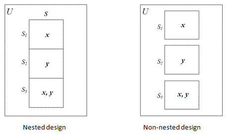
Description for Figure 2.1

We denote by $w_i$ the vector of design weights for sample $S_i,i=\mathrm{1,2,3},$ and by $X_i$ and $Y_i$ the sample matrices of $x$ and $y,$ the subscripts indicating the sample. We obtain simple Horvitz-Thompson (HT) estimators ${\widehat{X}}_1\left(={X^{\prime }}_1{w}_1\right)$ and ${\widehat{X}}_3$ of the population total $t_x$ of $x,$ using $S_1$ and $S_3,$ respectively, and HT estimators ${\widehat{Y}}_2$ and ${\widehat{Y}}_3$ of the total $t_y$ of $y,$ using $S_2$ and $S_3.$ For more efficient estimation of the totals $t_x$ and $t_y$ we seek composite estimators that combine all the available information on $x$ and $y$ in the three samples. Such composite estimators that are best linear unbiased estimators (BLUE), i.e., minimum-variance linear unbiased combinations of the four estimators ${\widehat{X}}_1,{\widehat{Y}}_2,{\widehat{X}}_3$ and ${\widehat{Y}}_3,$ are denoted by ${\widehat{X}}^B$ and ${\widehat{Y}}^B$ and given in matrix form by

$$\left(\begin{array}{c}{\widehat{X}}^B\\ {\widehat{Y}}^B\end{array}\right)=P\left(\begin{array}{c}{\widehat{X}}_1\\ {\widehat{Y}}_2\\ {\widehat{X}}_3\\ {\widehat{Y}}_3\end{array}\right)\mathrm{,}(2.1)$$

where $P={\left(W^{\prime }{V}^{-1}W\right)}^{-1}{W}^{\prime }{V}^{-1},$ the matrix $W$ satisfies $E\left[{\left({{\widehat{X}}^{\prime }}_1\mathrm{,}{{\widehat{Y}}^{\prime }}_2\mathrm{,}{{\widehat{X}}^{\prime }}_3\mathrm{,}{{\widehat{Y}}^{\prime }}_3\right)}^{\prime }\right]=W{\left({t^{\prime }}_x\mathrm{,}{t^{\prime }}_y\right)}^{\prime }$ and has entries $1’\text{s}$ and $0’\text{s,}$ and $V$ is the variance-covariance matrix of ${\left({{\widehat{X}}^{\prime }}_1\mathrm{,}{{\widehat{Y}}^{\prime }}_2\mathrm{,}{{\widehat{X}}^{\prime }}_3\mathrm{,}{{\widehat{Y}}^{\prime }}_3\right)}^{\prime }.$ This estimation method was proposed by Chipperfield and Steel (2009), who provided analytical expressions of the BLUE for scalars $x$ and $y$ in non-nested matrix sampling, assuming simple random sampling and known $V.$ Such an approach to composite estimation has been explored also in a different context of survey sampling; see Wolter (1979), Jones (1980) and Fuller (1990). In general, computation of the BLUE given by (2.1) is not at all practical, as the computation of an estimated matrix $V$ (and its inverse) in $P$ would be quite laborious, especially if the number of variables or the sizes of the samples were large; it would be prohibitive if estimates for subpopulations were also required. Of course, the problem would become more difficult with more samples involved.

A more practical formulation of this estimation procedure is as follows. First, we express the composite estimators in (2.1) explicitly as linear combinations of the HT estimators ${\widehat{X}}_1,{\widehat{Y}}_2,{\widehat{X}}_3$ and ${\widehat{Y}}_3,$ i.e.,

$$\begin{array}{lll}{\widehat{X}}^B\hfill & =\hfill & B_{1x}{\widehat{X}}_1+B_{2x}{\widehat{Y}}_2+B_{3x}{\widehat{X}}_3+B_{4x}{\widehat{Y}}_3\hfill \\ {\widehat{Y}}^B\hfill & =\hfill & B_{1y}{\widehat{X}}_1+B_{2y}{\widehat{Y}}_2+B_{3y}{\widehat{X}}_3+B_{4y}{\widehat{Y}}_3.\hfill \end{array}$$

The condition of unbiasedness, $E\left({\widehat{X}}^B\right)=t_x$ and $E\left({\widehat{Y}}^B\right)=t_y,$ implies that $B_{3x}=I-B_{1x},$ $B_{4x}=-B_{2x}$ and $B_{4y}=I-B_{2y},$ $B_{3y}=-B_{1y}.$ Thus, $P$ and $W$ can be expressed as

$$P=\left(\begin{array}{cccc}{B}_{1x}& B_{2x}& I-B_{1x}& -B_{2x}\\ B_{1y}& B_{2y}& -B_{1y}& I-B_{2y}\end{array}\right)\mathrm{,}{W}^{\prime }=\left(\begin{array}{cccc}I& 0& I& 0\\ 0& I& 0& I\end{array}\right)\mathrm{,}$$

respectively, and the two composite estimators have necessarily the regression form

 $$\begin{array}{lll}{\widehat{X}}^B\hfill & =\hfill & {\widehat{X}}_3+B_{1x}\left({\widehat{X}}_1-{\widehat{X}}_3\right)+B_{2x}\left({\widehat{Y}}_2-{\widehat{Y}}_3\right)\hfill \\ {\widehat{Y}}^B\hfill & =\hfill & {\widehat{Y}}_3+B_{1y}\left({\widehat{X}}_1-{\widehat{X}}_3\right)+B_{2y}\left({\widehat{Y}}_2-{\widehat{Y}}_3\right)\mathrm{.}\hfill \end{array}(2.2)$$

Then writing $P=\left(ℬ\mathrm{,}I-ℬ\right),$ in obvious notation for matrix $ℬ,$ we can express (2.1) as

$$\left(\begin{array}{c}{\widehat{X}}^B\\ {\widehat{Y}}^B\end{array}\right)=ℬ\left(\begin{array}{c}{\widehat{X}}_1\\ {\widehat{Y}}_2\end{array}\right)+\left(I-ℬ\right)\left(\begin{array}{c}{\widehat{X}}_3\\ {\widehat{Y}}_3\end{array}\right)=\left(\begin{array}{c}{\widehat{X}}_3\\ {\widehat{Y}}_3\end{array}\right)+ℬ\left(\begin{array}{c}{\widehat{X}}_1-{\widehat{X}}_3\\ {\widehat{Y}}_2-{\widehat{Y}}_3\end{array}\right)\mathrm{,}(2.3)$$

the right-hand side of (2.3) being the matrix form of (2.2). The problem of finding the optimal (variance-minimizing) $P$ of the BLUE in (2.1) reduces then to that of finding the optimal matrix $ℬ$ in (2.3). The estimated optimal ${\widehat{ℬ}}^o$ is given by

$${\widehat{ℬ}}^o=-\widehat{\text{Cov}}\left(\begin{array}{c}\left(\begin{array}{c}{\widehat{X}}_3\\ {\widehat{Y}}_3\end{array}\right)\mathrm{,}\left(\begin{array}{c}{\widehat{X}}_1-{\widehat{X}}_3\\ {\widehat{Y}}_2-{\widehat{Y}}_3\end{array}\right)\end{array}\right){\left[\widehat{V}\left(\begin{array}{c}{\widehat{X}}_1-{\widehat{X}}_3\\ {\widehat{Y}}_2-{\widehat{Y}}_3\end{array}\right)\right]}^{-1}\mathrm{,}(2.4)$$

and when the three samples are independent it reduces to

$${\widehat{ℬ}}^o=\widehat{V}\left(\begin{array}{c}{\widehat{X}}_3\\ {\widehat{Y}}_3\end{array}\right){\left[\widehat{V}\left(\begin{array}{c}{\widehat{X}}_1\\ {\widehat{Y}}_2\end{array}\right)+\widehat{V}\left(\begin{array}{c}{\widehat{X}}_3\\ {\widehat{Y}}_3\end{array}\right)\right]}^{-1}\mathrm{.}(2.5)$$

In view of (2.3), with such optimal ${\widehat{ℬ}}^o$ the estimated BLUE in (2.1) (involving the estimated $\widehat{V},$ and with $\widehat{P}=\left({\widehat{ℬ}}^o\mathrm{,}I-{\widehat{ℬ}}^o\right)$ is a special type of optimal multivariate regression estimator. For the form of the ordinary (single-sample) optimal regression estimator and relevant discussion, see Montanari (1987) and Rao (1994).

Expressing the estimated variance of the HT estimator of a total (see, for example, Särndal, Swensson and Wretman (1992), page 43) as a quadratic form with associated non-negative definite matrix ${\Lambda }^0=\left\{\left({\pi }_{kl}-{\pi }_k{\pi }_l\right)/{\pi }_k{\pi }_l{\pi }_{kl}\right\},$ where ${\pi }_k,{\pi }_{kl}$ are first-and-second order inclusion probabilities, it can be shown after some matrix algebra that

$${\widehat{ℬ}}^o=({{\mathcal{X}}^{\prime }}_3{\Lambda }^0\mathcal{X}){({\mathcal{X}}^{\prime }{\Lambda }^0\mathcal{X})}^{-1}\mathrm{,}(2.6)$$

where

$$\mathcal{X}=\left(\begin{array}{cc}-X_1& 0\\ 0& -Y_2\\ X_3& Y_3\end{array}\right)(2.7)$$

is the $n\times \left(p+q\right)$ design matrix corresponding to the regression estimator (2.3), ${\mathcal{X}}_3$ is the matrix $\mathcal{X}$ with the first two rows set equal to zero, and ${\Lambda }^0$ is associated with the combined sample $S=S_1\cup S_2\cup S_3,$ reducing in the non-nested sampling to the block-diagonal matrix $\text{diag}\left\{{\Lambda }_i^0\right\}$ with ${\Lambda }_i^0$ associated with the sample $S_i.$ For the nested design, the probabilities defining ${\Lambda }^0$ are products of the probabilities of inclusion in $S$ and the conditional (on $S$ ) subsampling probabilities. With this estimated ${\widehat{ℬ}}^o,$ the estimated BLUE in (2.3), called composite optimal regression estimator (COR) and denoted by ${\widehat{\mathcal{X}}}^{\text{COR}},$ is written compactly as ${\widehat{\mathcal{X}}}^{\text{COR}}={\widehat{\mathcal{X}}}_3-{\widehat{ℬ}}^o\widehat{\mathcal{X}}[={({\mathcal{X}}_3-\mathcal{X}{\widehat{ℬ}}^{o^{\prime }})}^{\prime }w],$ where $w={\left({w^{\prime }}_1\mathrm{,}{w^{\prime }}_2\mathrm{,}{w^{\prime }}_3\right)}^{\prime }$ is the vector of design weights of the combined sample $S.$ It transpires that the COR estimator is in fact the sum of weighted sample regression residuals, and ${\widehat{ℬ}}^o$ minimizes the quadratic form ${\left({\mathcal{X}}_3-\mathcal{X}{\widehat{ℬ}}^{o^{\prime }}\right)}^{\prime }$ ${\Lambda }^0\left({\mathcal{X}}_3-\mathcal{X}{\widehat{ℬ}}^{o^{\prime }}\right)$ in these residuals, which is the estimated approximate (large-sample) variance of ${\widehat{\mathcal{X}}}^{\text{COR}}.$

Now, upon writing ${\widehat{\mathcal{X}}}^{\text{COR}}$ as ${\widehat{\mathcal{X}}}^{\text{COR}}={{\mathcal{X}}^{\prime }}_3\left[w+{\Lambda }^0\mathcal{X}{\left({\mathcal{X}}^{\prime }{\Lambda }^0\mathcal{X}\right)}^{-1}\left(0-{\mathcal{X}}^{\prime }w\right)\right],$ it appears that the COR estimator has the form of a calibration estimator (with vector of calibration totals $0={\left(0^{\prime }\mathrm{,}{0}^{\prime }\right)}^{\prime }$ of dimension $\left(p+q\right)),$ whose components satisfy the constraints ${\widehat{X}}_1^{\text{COR}}={\widehat{X}}_3^{\text{COR}}$ and ${\widehat{Y}}_2^{\text{COR}}={\widehat{Y}}_3^{\text{COR}},$ i.e., calibrated estimates of the same total from two different samples are equal. Indeed, the vector

$$c=w+{\Lambda }^0\mathcal{X}{\left({\mathcal{X}}^{\prime }{\Lambda }^0\mathcal{X}\right)}^{-1}\left(0-{\mathcal{X}}^{\prime }w\right)\mathrm{,}(2.8)$$

is the vector of calibrated weights that minimizes the generalized least-squares distance ${\left(c-w\right)}^{\prime }{\left({\Lambda }^0\right)}^{-1}\left(c-w\right)$ while satisfying the constraints ${X^{\prime }}_1{c}_1={X^{\prime }}_3{c}_3$ and ${Y^{\prime }}_2{c}_2={Y^{\prime }}_3{c}_3,$ where the subcector $c_i$ corresponds to sample $S_i.$ This follows from a general result for the single-sample case, according to which calibration with the generalized least-squares distance measure may involve an arbitrary $n\times n$ positive definite matrix $R$ instead of ${\Lambda }^0;$ see Andersson and Thorburn (2005).

We may now write the COR estimator formally as a calibration estimator, ${\widehat{\mathcal{X}}}^{\text{COR}}={{\mathcal{X}}^{\prime }}_{3}c,$ and using the subvector of calibrated weights $c_3,$ for sample $S_3$ only, we obtain the components of ${\widehat{\mathcal{X}}}^{\text{COR}}$ directly in the simple linear forms

$${\widehat{X}}^{\text{COR}}={X^{\prime }}_3{c}_3={\displaystyle {\sum }_{S_3}{c}_k{x}_k};{\widehat{Y}}^{\text{COR}}={Y^{\prime }}_3{c}_3={\displaystyle {\sum }_{S_3}{c}_k{y}_k}\mathrm{,}$$

as in common survey practice. Yet, a decomposition of the vector $c$ based on the following general lemma on calibration gives an analytic expression of ${\widehat{X}}^{\text{COR}}$ and ${\widehat{Y}}^{\text{COR}}$ of the form (2.2), which provides insight into the structure and the efficiency of the COR estimator. The proof of the lemma is given in the Appendix.

Lemma 1 Let $\mathcal{X}$ be a design matrix of dimension $n\times \left(p+q\right)$ and of full rank and written in partition form $\left(X\mathrm{,}\Psi \right),$with corresponding vector of calibration totals $t_{\mathcal{X}}={\left({t^{\prime }}_X\mathrm{,}{t^{\prime }}_{\Psi }\right)}^{\prime },$ and let $R$ be any positive definite matrix of dimension $n\times n.$ Then the vector of calibrated weights $c=w+R\mathcal{X}{\left({\mathcal{X}}^{\prime }R\mathcal{X}\right)}^{-1}$  $\left(t_{\mathcal{X}}-{\mathcal{X}}^{\prime }w\right),$ obtained from the calibration procedure involving the distance measure ${\left(c-w\right)}^{\prime }{R}^{-1}$  $\left(c-w\right)$ and the constraint ${\mathcal{X}}^{\prime }c=t_{\mathcal{X}},$ can be decomposed as

$$c=w+L_{\Psi }X{\left(X^{\prime }{L}_{\Psi }X\right)}^{-1}\left[t_X-X^{\prime }w\right]+L_X\Psi {\left({\Psi }^{\prime }{L}_X\Psi \right)}^{-1}\left[t_{\Psi }-{\Psi }^{\prime }w\right]\mathrm{,}(2.9)$$

where $L_X=R\left(I-P_X\right)$ with $P_X=X{\left(X^{\prime }RX\right)}^{-1}{X}^{\prime }R,$ and $L_{\Psi }=R\left(I-P_{\Psi }\right)$ with $P_{\Psi }=\Psi {\left({\Psi }^{\prime }R\Psi \right)}^{-1}{\Psi }^{\prime }R.$ The vector $c$ can be written as

$$c=c_{\Psi }+L_{\Psi }X{\left(X^{\prime }{L}_{\Psi }X\right)}^{-1}\left[t_X-X^{\prime }{c}_{\Psi }\right]\mathrm{,}(2.10)$$

where the vector

$$c_{\Psi }=w+R\Psi {\left({\Psi }^{\prime }R\Psi \right)}^{-1}\left[t_{\Psi }-{\Psi }^{\prime }w\right]$$

is generated by calibration of the design weights involving only $\Psi$ and $t_{\Psi }.$ By symmetry,

$$c=c_X+L_X\Psi {\left({\Psi }^{\prime }{L}_X\Psi \right)}^{-1}\left[t_{\Psi }-{\Psi }^{\prime }{c}_X\right]\mathrm{,}(2.11)$$

where

$$c_X=w+RX{\left(X^{\prime }RX\right)}^{-1}\left[t_X-X^{\prime }w\right]\mathrm{.}$$

Now, if $\mathcal{X}$ is as in (2.7), with corresponding vector of calibration totals $t_{\mathcal{X}}={\left(0^{\prime }\mathrm{,}{0}^{\prime }\right)}^{\prime },$ and if $R={\Lambda }^0,$ then it follows from (2.9) that (2.8) can be written in the form

$$c=w+L_{\Psi }X{\left(X^{\prime }{L}_{\Psi }X\right)}^{-1}\left[{\widehat{X}}_1-{\widehat{X}}_3\right]+L_X\Psi {\left({\Psi }^{\prime }{L}_X\Psi \right)}^{-1}\left[{\widehat{Y}}_2-{\widehat{Y}}_3\right]\mathrm{,}$$

and thus

$$\begin{array}{lll}{\widehat{X}}^{\text{COR}}\hfill & =\hfill & {X^{\prime }}_3{c}_3={\widehat{X}}_3+{\widehat{B}}_{1x}^o\left({\widehat{X}}_1-{\widehat{X}}_3\right)+{\widehat{B}}_{2x}^o\left({\widehat{Y}}_2-{\widehat{Y}}_3\right)\hfill \\ \hfill & =\hfill & {\widehat{B}}_{1x}^o{\widehat{X}}_1+\left(I-{\widehat{B}}_{1x}^o\right){\widehat{X}}_3+{\widehat{B}}_{2x}^o\left({\widehat{Y}}_2-{\widehat{Y}}_3\right)\mathrm{,}(2.12)\hfill \end{array}$$

in obvious notation for ${\widehat{B}}_{1x}^o$ and ${\widehat{B}}_{2x}^o.$ A similar expression is obtained for ${\widehat{Y}}^{\text{COR}}.$ It is seen from (2.12) that the COR estimator ${\widehat{X}}^{\text{COR}}$ of $t_x$ is approximately (for large samples) unbiased, and derives its efficiency from combining the two elementary estimators ${\widehat{X}}_1$ and ${\widehat{X}}_3$ (pooling information from samples $S_1$ and $S_3)$ and from borrowing strength from sample $S_2$ through the correlation between $x$ and $y.$ In view of (2.10), the estimator ${\widehat{X}}^{\text{COR}}$ takes the alternative forms

$$\begin{array}{lll}{\widehat{X}}^{\text{COR}}\hfill & =\hfill & {X^{\prime }}_3{c}_{3\Psi }+{X^{\prime }}_3{L}_{\Psi }X{\left(X^{\prime }{L}_{\Psi }X\right)}^{-1}\left[{X^{\prime }}_1{c}_{1\Psi }-{X^{\prime }}_3{c}_{3\Psi }\right]\hfill \\ \hfill & =\hfill & {\widehat{X}}_3^{\text{OR}}+{\widehat{B}}_{1x}^o\left[{\widehat{X}}_1^{\text{OR}}-{\widehat{X}}_3^{\text{OR}}\right]\hfill \\ \hfill & =\hfill & {\widehat{B}}_{1x}^o{\widehat{X}}_1^{\text{OR}}+\left(I-{\widehat{B}}_{1x}^o\right){\widehat{X}}_3^{\text{OR}}\mathrm{,}(2.13)\hfill \end{array}$$

where ${\widehat{X}}_i^{\text{OR}}={\widehat{X}}_i+{X^{\prime }}_i{\Lambda }^0\Psi {\left({\Psi }^{\prime }{\Lambda }^0\Psi \right)}^{-1}\left({\widehat{Y}}_2-{\widehat{Y}}_3\right)$ are optimal regression (OR) estimators incorporating the regression effect of the last term in (2.12).

In non-nested matrix sampling, ${\Lambda }^0=\text{diag}\left\{{\Lambda }_i^0\right\},$ ${\widehat{X}}_1^{\text{OR}}={\widehat{X}}_1,$ ${\widehat{X}}_3^{\text{OR}}={\widehat{X}}_3+\widehat{\text{Cov}}({\widehat{X}}_3\mathrm{,}{\widehat{Y}}_3){[\widehat{V}({\widehat{Y}}_2)+\widehat{V}({\widehat{Y}}_3)]}^{-1}[{\widehat{Y}}_2-{\widehat{Y}}_3],$ having estimated approximate variance $\widehat{\text{AV}}\left({\widehat{X}}_3^{\text{OR}}\right)=\widehat{V}\left({\widehat{X}}_3\right)-\widehat{\text{Cov}}\left({\widehat{X}}_3\mathrm{,}{\widehat{Y}}_3\right){\left[\widehat{V}\left({\widehat{Y}}_2\right)+\widehat{V}\left({\widehat{Y}}_3\right)\right]}^{-1}{\widehat{\text{Cov}}}^{\prime }\left({\widehat{X}}_3\mathrm{,}{\widehat{Y}}_3\right),$ and ${\widehat{B}}_{1x}^o=\widehat{\text{AV}}\left({\widehat{X}}_3^{\text{OR}}\right){\left[\widehat{V}\left({\widehat{X}}_1\right)+\widehat{\text{AV}}\left({\widehat{X}}_3^{\text{OR}}\right)\right]}^{-1}$ is the coefficient that minimizes the variance $\widehat{\text{AV}}\left({\widehat{X}}^{\text{COR}}\right).$ From the explicit form $I-{\widehat{B}}_{1x}^o=\widehat{V}\left({\widehat{X}}_1\right){\left[\widehat{V}\left({\widehat{X}}_1\right)+\widehat{V}\left({\widehat{X}}_3\right)-\widehat{\text{Cov}}\left({\widehat{X}}_3\mathrm{,}{\widehat{Y}}_3\right)\times {\left[\widehat{V}\left({\widehat{Y}}_2\right)+\widehat{V}\left({\widehat{Y}}_3\right)\right]}^{-1}{\widehat{\text{Cov}}}^{\prime }\left({\widehat{X}}_3\mathrm{,}{\widehat{Y}}_3\right)\right]}^{-1},$ it is then clear that the stronger the correlation between $x$ and $y$ the larger the $I-{\widehat{B}}_{1x}^o$ and more weight is given to the less variable component ${\widehat{X}}_3^{\text{OR}}.$ In this connection, it can be easily shown that $\widehat{\text{AV}}\left({\widehat{X}}^{\text{COR}}\right)$ satisfies

$$\widehat{\text{AV}}\left({\widehat{X}}^{\text{COR}}\right){\left[\widehat{V}\left({\widehat{X}}_1\right)\right]}^{-1}={\widehat{B}}_{1x}^o\text{<}I\mathrm{,}\widehat{\mathrm{AV}}\left({\widehat{X}}^{\text{COR}}\right){\left[\widehat{\mathrm{AV}}\left({\widehat{X}}_3^{\text{OR}}\right)\right]}^{-1}=I-{\widehat{B}}_{1x}^o\text{<}I\mathrm{.}$$

These inequalities hold also for any linear combination of the components of each of the estimators involved. The optimal composite regression estimator ${\widehat{X}}^{\text{COR}}$ is more efficient than each of its two components ${\widehat{X}}_1$ and ${\widehat{X}}_3^{\text{OR}}$ by the shown quantities, with the efficiency depending on the strength of the correlation between $x$ and $y.$ The estimator ${\widehat{X}}^{\text{COR}}$ is also more efficient than the estimator ${\tilde{X}}^{\text{COR}}={\tilde{B}}_{1x}^o{\widehat{X}}_1+\left(I-{\tilde{B}}_{1x}^o\right){\widehat{X}}_3,$ with ${\tilde{B}}_{1x}^o=\widehat{V}\left({\widehat{X}}_3\right){\left[\widehat{V}\left({\widehat{X}}_1\right)+\widehat{V}\left({\widehat{X}}_3\right)\right]}^{-1},$ which does not incorporate the information on $y$ (does not borrow strength from sample $S_2)$ and has estimated variance $\widehat{\text{AV}}\left({\tilde{X}}^{\text{COR}}\right)=\widehat{V}\left({\widehat{X}}_1\right){\left[\widehat{V}\left({\widehat{X}}_1\right)+\widehat{V}\left({\widehat{X}}_3\right)\right]}^{-1}\widehat{V}\left({\widehat{X}}_3\right).$ Indeed, writing the variance $\widehat{\text{AV}}\left({\widehat{X}}^{\text{COR}}\right)=\widehat{V}\left({\widehat{X}}_1\right){\widehat{B}}_{1x}^o$ as $\widehat{\text{AV}}\left({\widehat{X}}^{\text{COR}}\right)=\widehat{V}\left({\widehat{X}}_1\right){\left[\widehat{V}\left({\widehat{X}}_1\right)+\widehat{V}\left({\widehat{X}}_3\right)\right]}^{-1}\widehat{V}\left({\widehat{X}}_3\right)E,$ where $E=E_1{E}_2$ with $E_1=[I-{(\widehat{V}({\widehat{X}}_3))}^{-1}\widehat{\text{Cov}}({\widehat{X}}_3\mathrm{,}{\widehat{Y}}_3){[\widehat{V}({\widehat{Y}}_2)+\widehat{V}({\widehat{Y}}_3)]}^{-1}{\widehat{\text{Cov}}}^{\prime }({\widehat{X}}_3\mathrm{,}{\widehat{Y}}_3)]$ and $E_2={[I-{[\widehat{V}({\widehat{X}}_1)+\widehat{V}({\widehat{X}}_3)]}^{-1}\widehat{\text{Cov}}({\widehat{X}}_3\mathrm{,}{\widehat{Y}}_3){[\widehat{V}({\widehat{Y}}_2)+\widehat{V}({\widehat{Y}}_3)]}^{-1}{\widehat{\text{Cov}}}^{\prime }({\widehat{X}}_3\mathrm{,}{\widehat{Y}}_3)]}^{-1},$ and noticing that $E\le I,$ it follows that

$$\widehat{\text{AV}}\left({\widehat{X}}^{\text{COR}}\right){\left[\widehat{\text{AV}}\left({\tilde{X}}^{\text{COR}}\right)\right]}^{-1}=E\le I\mathrm{,}$$

that is, borrowing strength from $S_2$ reduces the variance of the composite estimator of $t_x$ by the factor $E,$ which depends on the strength of the correlation between $x$ and $y.$ It can be easily verified that for two scalar variables $x$ and $y$ and simple random sampling this result reduces to the analogous analytical result on the efficiency of BLUE given in Chipperfield and Steel (2009, page 231). In this simple case $E=\left[n_1+n_3\right]\left[n_3+n_2\left(1-{\rho }^2\right)\right]/\left[\left(n_1+n_3\right)\left(n_2+n_3\right)-n_1{n}_2{\rho }^2\right],$ where $\rho$ is the correlation between $x$ and $y.$ As an illustration, assuming equal sample sizes and correlation $\rho =0.7,$ the efficiency gain is 13.96%.

In nested matrix sampling, the two estimators in (2.13) are ${\widehat{X}}_i^{\text{OR}}={\widehat{X}}_i+\widehat{\text{Cov}}\left({\widehat{X}}_i\mathrm{,}\widehat{\Psi }\right){\left[\widehat{V}\left(\widehat{\Psi }\right)\right]}^{-1}\left[{\widehat{Y}}_2-{\widehat{Y}}_3\right],$ and ${\widehat{B}}_{1x}^o=[\widehat{\text{AV}}({\widehat{X}}_3^{\text{OR}})-\widehat{\text{AC}}({\widehat{X}}_1^{\text{OR}}\mathrm{,}{\widehat{X}}_3^{\text{OR}})]{[\widehat{\text{AV}}({\widehat{X}}_1^{\text{OR}})+\widehat{\text{AV}}({\widehat{X}}_3^{\text{OR}})-2\widehat{\text{AC}}({\widehat{X}}_1^{\text{OR}}\mathrm{,}{\widehat{X}}_3^{\text{OR}})]}^{-1},$ where AC denotes approximate covariance. In this case, in addition to the correlation ${\rho }_{x\mathrm{3,}y3}$ between ${\widehat{X}}_3$ and ${\widehat{Y}}_3$ in sample $S_3,$ the efficiency of ${\widehat{X}}^{\text{COR}}$ depends on the estimators' correlations ${\rho }_{x\mathrm{1,}x3},{\rho }_{y\mathrm{2,}y3},{\rho }_{y\mathrm{2,}x3}$ due to the dependence of the subsamples. For univariate $x$ and $y$ and with the simplifying assumption of identical designs for the three subsamples (as in equal splitting of the full sample), we obtain some insight through the simple expressions $\widehat{\text{AV}}\left({\widehat{X}}^{\text{COR}}\right)=V\left({\widehat{X}}_3\right)\left[2\left(1-{\rho }_{x\mathrm{1,}x3}^2\right)\left(1-{\rho }_{y\mathrm{2,}y3}\right)-{\left({\rho }_{x\mathrm{3,}y3}-{\rho }_{y\mathrm{2,}x3}\right)}^2\right]/\left[4\left(1-{\rho }_{x\mathrm{1,}x3}\right)\left(1-{\rho }_{y\mathrm{2,}y3}\right)-{\left({\rho }_{x\mathrm{3,}y3}-{\rho }_{y\mathrm{2,}x3}\right)}^2\right],$ and $\widehat{\text{AV}}\left({\tilde{X}}^{\text{COR}}\right)=V\left({\widehat{X}}_3\right)\left(1+{\rho }_{x\mathrm{1,}x3}\right)/2.$ Clearly, the estimator ${\tilde{X}}^{\text{COR}},$ which ignores information on $y,$ is more efficient than the simple average of single-sample estimators of $t_x$ only when there is negative correlation ${\rho }_{x\mathrm{1,}x3}.$ The efficiency of ${\widehat{X}}^{\text{COR}}$ relative to ${\tilde{X}}^{\text{COR}}$

$$\frac{\widehat{\text{AV}}\left({\widehat{X}}^{\text{COR}}\right)}{\widehat{\text{AV}}\left({\tilde{X}}^{\text{COR}}\right)}=\frac{4\left(1-{\rho }_{x\mathrm{1,}x3}^2\right)\left(1-{\rho }_{y\mathrm{2,}y3}\right)-2{\left({\rho }_{x\mathrm{3,}y3}-{\rho }_{y\mathrm{2,}x3}\right)}^2}{4\left(1-{\rho }_{x\mathrm{1,}x3}^2\right)\left(1-{\rho }_{y\mathrm{2,}y3}\right)-\left(1+{\rho }_{x\mathrm{1,}x3}\right){\left({\rho }_{x\mathrm{3,}y3}-{\rho }_{y\mathrm{2,}x3}\right)}^2}$$

depends on the sign and size of ${\rho }_{x\mathrm{1,}x3}$ and the size of $\left|{\rho }_{x\mathrm{3,}y3}-{\rho }_{y\mathrm{2,}x3}\right|.$

Although the calibration procedure, with vector of calibrated weights (2.8), substantially facilitates the computation of the composite optimal regression estimator for any total of interest, the matrix ${\Lambda }^0$ makes the calculations exceedingly demanding, particularly in nested sampling where the subsamples are dependent and thus ${\Lambda }^0$ is not diag $\left\{{\Lambda }_i^0\right\}.$ Besides, the probabilities ${\pi }_{kl}$ are not known for most sampling designs. An alternative composite regression estimator that is computationally very efficient is developed in the next section.

Previous | Next