
Register-based sampling for household panels 7. Application
In the RIS, core persons are selected from the population aged 15 years and older through stratified simple random sampling without replacement with a sample fraction of 0.16. In this application results are presented for a large municipality (Rotterdam), a municipality of intermediate size (Enschede) and a small municipality (Sevenum) for three consecutive years 2006, 2007 and 2008. Population and sample sizes for these three municipalities are summarized in Table 7.1.
| Municipality | Population | Sample | |||
|---|---|---|---|---|---|
| Households | Persons 15 and older | Core persons | Unique households | Unique persons | |
| Rotterdam | 293,400 | 484,000 | 73,000 | 67,600 | 171,400 |
| Enschede | 74,200 | 128,000 | 19,300 | 17,600 | 46,300 |
| Sevenum | 2,950 | 6,100 | 870 | 750 | 2,500 |
Target variables of interest for the RIS are:
- Income distribution of households in ten classes where the categories are based on ten percentage point quantiles (deciles) of the national distribution using standardized household income (abbreviated as IncDistHh);
- Mean standardized household income (abbreviated as HHinc);
- Mean disposable income of persons that receive income during the 52 weeks of the year (abbreviated as Pinc).
Disposable income of a person is total income of a person minus his or her current taxes. Total income contains earnings, profit, income from capital and savings, and social or other benefits. Standardized household income is defined as the total disposable income of a household corrected for differences in household size and composition. In the literature, this is also known as the equivalised spendable income (OECD 2013).
Estimates for official publications of the RIS are obtained with the GREG estimator using the method of Lemaître and Dufour (1987). Since this survey does not suffer from nonresponse, auxiliary information is used in the estimation for variance reduction and consistency between the marginals of different publication tables. Inclusion expectations are based on the formulas derived in Subsection 3.1. For each municipality the following weighting scheme is applied in the GREG estimator:
All auxiliary variables are categorical. The numbers between brackets denote the number of categories. MaritalStatus distinguishes between people who are married and other forms of marital status. Address distinguishes between addresses where one family is residing and other types of addresses. HHsize stands for household size and distinguishes between households with one, two, three, four, and five or more persons. Estimates for HHinc and Pinc with their standard errors based on the HT estimator, the GREG estimator and the GREG estimator with the method of Lemaître and Dufour (1987) are given in Table 7.2. In Figure 7.1 the income distributions IncDistHh estimated with the HT estimator, GREG estimator and the GREG estimator with the method of Lemaître and Dufour (1987) are plotted with a 95% confidence interval for Rotterdam and Sevenum in 2008. The standard errors for these estimates are compared in a separate histogram. In Figure 7.2 the IncDistHh for Rotterdam and Sevenum estimated with the method of Lemaître and Dufour (1987) are given for 2006, 2007 and 2008. See van den Brakel (2013) for more detailed output of the income distributions.
| Variable | Year | HT | GREG | GREG consistent (L&D) | ||||
|---|---|---|---|---|---|---|---|---|
| Rotterdam | HHinc | 2006 | 19,790 | (83) | 20,134 | (80) | 20,161 | (76) |
| 2007 | 22,306 | (73) | 22,950 | (64) | 22,866 | (64) | ||
| 2008 | 23,750 | (78) | 24,511 | (69) | 24,410 | (68) | ||
| Pinc | 2006 | 22,074 | (94) | 22,219 | (84) | 22,233 | (93) | |
| 2007 | 24,094 | (82) | 24,362 | (75) | 24,432 | (78) | ||
| 2008 | 25,325 | (84) | 25,625 | (75) | 25,705 | (78) | ||
| Enschede | HHinc | 2006 | 19,810 | (128) | 20,353 | (111) | 20,300 | (107) |
| 2007 | 20,878 | (128) | 21,716 | (107) | 21,753 | (105) | ||
| 2008 | 22,254 | (148) | 23,235 | (125) | 23,237 | (123) | ||
| Pinc | 2006 | 20,402 | (102) | 20,608 | (92) | 20,590 | (92) | |
| 2007 | 21,387 | (115) | 21,751 | (103) | 21,852 | (106) | ||
| 2008 | 22,235 | (123) | 22,659 | (110) | 22,724 | (114) | ||
| Sevenum | HHinc | 2006 | 25,696 | (799) | 25,698 | (734) | 25,968 | (711) |
| 2007 | 28,207 | (618) | 28,901 | (520) | 29,026 | (490) | ||
| 2008 | 31,466 | (795) | 32,372 | (715) | 32,536 | (694) | ||
| Pinc | 2006 | 21,328 | (466) | 21,680 | (428) | 21,712 | (428) | |
| 2007 | 24,056 | (456) | 24,219 | (396) | 24,459 | (393) | ||
| 2008 | 24,980 | (468) | 25,482 | (426) | 25,644 | (455) | ||
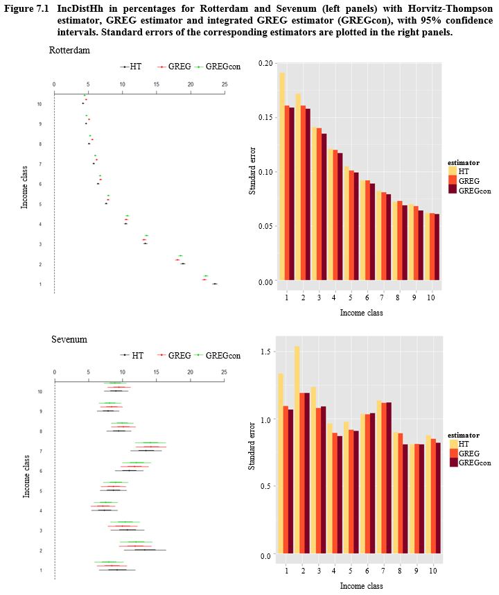
Description of Figure 7.1
Figure made of four graphs, namely the income distribution of households in percentages for Rotterdam and Sevenum with Horvitz-Thompson estimator, GREG estimator and integrated GREG estimator (GREGcon), with 95% confidence intervals and a bar chart of standard errors of the corresponding estimators for each city.
For Rotterdam (first graph), the income distribution of households in percentages is on the y-axis going from 5% to 25% and the income classes are on the x-axis going from 10 to 1. The three estimators are close. Their confidence intervals are narrow. Class 10 represents about 5% of the incomes. The percentage increases when the class decreases to about 25% of the incomes for class 1. The bar chart (second graph) presents the estimator standard errors on the y-axis going from 0.00 to 0.20. Income classes from 1 to 10 are on the x-axis. Standard error decreases when class increases. The standard error of the HT estimator seems to be generally greater than the standard error of the other two estimators. The standard error of the integrated GREG estimator seems to be lower.
For Sevenum (third graph), the income distribution of households in percentages is on the y-axis going from 5% to 20% and the income classes are on the x-axis going from 10 to 1. The three estimators are close. Their confidence intervals are wider. Each of the higher classes (8 to 10) represents about 10% of the incomes. The percentage increases to about 15% for class 7 before decreasing below 10% for class 4. Percentages increase slightly for classes 1 to 3, remaining below 15%. The bar chart (fourth graph) presents the estimator standard errors on the y-axis going from 0.0 to 1.5. Income classes from 1 to 10 are on the x-axis. For classes 1 to 4, standard error decreases when class increases. Standard error increases for classes 5 to 7 before decreasing for classes 8 to 10. The standard error of the HT estimator seems to be generally greater than the standard error of the other two estimators. The standard error of the integrated GREG estimator seems to be lower.
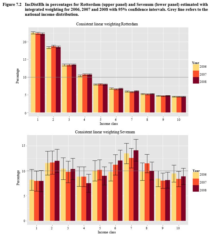
Description of Figure 7.2
Figure made of two bar charts, namely the income distribution of households in percentages for Rotterdam and Sevenum estimated with integrated weighting for 2006, 2007 and 2008 with 95% confidence intervals. For Rotterdam, the percentage is on the y-axis, going from 0 to 25 and the income classes from 1 to 10 are on the x-axis. Distributions are similar from one year to another, decreasing when the class increases. Confidence intervals are narrow. For Sevenum, the percentage is on the y-axis, going from 0 to 15 and the income classes from 1 to 10 are on the x-axis. The global behavior of the distributions is as described in Figure 7.2, rather similar from one year to another. Confidence intervals are wider.
The observed income distributions in Figures 7.1 and 7.2 are a result of the demographic compositions in both municipalities. Rotterdam is a city where the fraction of households in low income categories are above the national average, since the fractions in the first three categories are above 10%. The fraction of households in higher income categories, on the other hand, are below the national average, since these fractions are below 10%. This is a typical distribution for a large university city with a high fraction of non-western immigrants. Sevenum on the other hand is a small village close to a large industrial city. Such villages typically have small fractions of immigrants, no students and large fractions of households with one or two people that receive income during 52 weeks of the year. This explains why the fraction of households in the lowest income category is below the national average and the fraction of households in the higher income categories (6, 7 and 8) is above the national average. Sevenum is a village that does not attract extreme rich households.
Since HHinc and Pinc are based on different income definitions and since Pinc is the average over the domains of people that receive income during 52 weeks of the year, the differences between the two means vary between municipalities. For a large university city like Rotterdam, the mean standardized household income is typically smaller compared to the mean of disposable personal income averaged over people that receive income during 52 weeks of the year. Other cities with large universities show a similar picture. In a small but rich village like Sevenum, the situation is the other way around.
Another remarkable result is that in Rotterdam and Enschede the difference between the HT estimator and the GREG estimator is relatively large compared to the standard errors. Given the large sample size and the fact that there is no nonresponse, these differences are expected to be smaller. A possible explanation is that Rotterdam and Enschede are large university cities. Students are often identified in the tax register (used as the sample frame) in a different way than they appear in the population register (used to derive population distributions of the auxiliary variables), in particular with respect to their household situation.
For each municipality there is a steady increase over time in the mean of the income for households and persons. Also the income distributions for each municipality show a stable pattern over the years. This can be expected if a panel is applied in combination with large sample sizes to estimate phenomena that are not very volatile in time.
Comparing GREG estimates with and without using the method of Lemaître and Dufour (1987) shows that standard errors of estimated household parameters are smaller if the method of Lemaître and Dufour (1987) is applied. This is particularly visible for the mean household income in the small sample of Sevenum. For estimated person based parameters, on the other hand, the method of Lemaître and Dufour (1987) slightly increases the standard error compared to the regular GREG estimator. This suggests that the assumed variance structure for the residuals in the underlying regression model in the case of integrated weighting better fits the household-based variables than the person-based variables.
- Date modified: