
Publications
Population and Family Estimation Methods at Statistics Canada
Chapter 1
Postcensal and intercensal population estimates, Canada, provinces and territories

Archived Content
Information identified as archived is provided for reference, research or recordkeeping purposes. It is not subject to the Government of Canada Web Standards and has not been altered or updated since it was archived. Please "contact us" to request a format other than those available.
1.1 Postcensal population estimates, Canada, provinces and territories
1.2 Intercensal population estimates, Canada, provinces and territories
This chapter describes the types of method used by Statistics Canada to calculate postcensal and intercensal estimates for the total population and for the population by age and sex, at the provincial and territorial levels. The sources of data used to produce these estimates are also given.
1.1 Postcensal population estimates, Canada, provinces and territories
1.1.1 Definition and calculation of provincial and territorial postcensal estimates of total population
Postcensal population estimates are produced using data from the most recent census (adjusted for census net undercoverage (CNU)1 ) and estimates of the components of demographic growth since that census. The data are forwarded from the Census Day to July 1 by taking into account the components of demographic growth between Census Day and June 30 of the census year. The component method used to produce postcensal estimates is a population accounting system, where modifications are made to the current census population adjusted for CNU or most recent estimate by adding and subtracting the components of demographic growth that occur between July 1 and the reference date of the estimate.
The factors of demographic growth and their components are:
Natural increase
- births
- deaths
International migration
- immigrants
- emigrants
- returning emigrants
- net temporary emigration
- net non-permanent residents
Interprovincial migration
- in-migrants
- out-migrants
These components can also be divided into two groups, according to the type of data used: those components for which data are readily available, such as births, deaths, and immigration, and those that have to be estimated, such as interprovincial migration, emigrants, returning emigrants, net temporary emigration, and net non-permanent residents (NPRs).
The two components of natural increase, i.e. births and deaths, have similar methodological approach when it comes to estimation. Provincial and territorial Vital Statistics Acts (or equivalent legislation) render compulsory the registration of all live births and deaths within their jurisdictions. Vital statistics universe include births and deaths of all Canadians, immigrants and non-permanent residents (NPR) and exclude foreign residents.
Growth due to international migration represents the movement of population between Canada and a foreign country which involves a change in the usual place of residence.
Figure 1.1
International migration flows for Canada
Description for figure 1.1
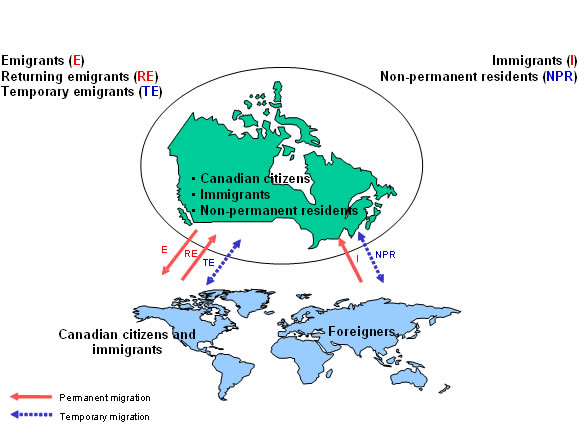
In the Demographic Estimates Program, international migration consists of five components: immigration, emigration, returning emigrants, net temporary emigration and net non-permanent residents. International migration flows can be categorized as either permanent or temporary. Permanent flows are composed of persons arriving in Canada for permanent residence (landed immigrants), Canadian citizens or immigrants returning to Canada after previously emigrated from Canada (returning emigrants), and Canadian citizens or immigrants leaving Canada to establish a permanent residence in another country (emigrants). Temporary flows relate to foreigners arriving for temporary stay in Canada and leaving after their stay ends (non-permanent residents), as well as Canadian citizens and immigrants living temporarily abroad who have not maintained a usual place of residence in Canada (temporary emigration).
Net non-permanent residents represent the variation in the number of non-permanent residents between two dates, and net temporary emigration represents the variation in the number of temporary emigrants between two dates. Different methodological approaches are used; one for the immigration component, another one for non-permanent residents and a more model based approach for the remaining components of international migration (emigration, returning emigrants, and net temporary emigration).
Finally, the last factor of demographic growth that is discussed is the interprovincial migration. While this factor does not affect the total Canadian population it does affect the provincial and territorial population counts and is a significant challenge for the Demographic Estimates Program.
Table 1.1 shows the sources and references of component data used to generate the postcensal population.
| Component | Sources and references (if applicable) |
|---|---|
| Base population | May 16, 2006 Census population adjusted for census net undercoverage and incompletely enumerated Indian reserves. 2006 Census: Statistics Canada, Census of Canada, 2006, Catalogue no. 92-200-XPB. |
| Census net undercoverage: See The Daily, September 29, 2008. Incompletely enumerated Indian reserves: See The Daily, September 29, 2008. |
|
| Births and deaths | Statistics Canada, Health Statistics Division. |
| Statistics Canada, Demography Division, Catalogue no. 91-215-X, annual, Catalogue no. 91-002-X, quarterly. | |
| Immigration | Citizenship and Immigration Canada (CIC). |
| Emigrants | Statistics Canada, Demography Division—from data on emigrant children from the Canada Child Tax Benefit program (CCTB) from Canada Revenue Agency files (CRA) and data from the U.S. Department of Homeland Security, Office of Immigration Statistics. |
| Returning emigrants | Statistics Canada, Demography Division—based on data from the CCTB program and adjustment factors calculated using CRA files. |
| Net temporary emigrants | Statistics Canada, Demography Division—based on data from the Reverse Record Check (RRC), 2001 and 2006 Censuses of Canada. |
| Non-permanent residents | Statistics Canada, Demography Division—based on data provided by Citizenship and Immigration Canada. |
| Interprovincial migration | Statistics Canada, Demography Division—based on the CCTB program and adjustment factors calculated using CRA files. |
Estimates of population are first produced for each province and territory, and then summed to obtain an estimate of the population of Canada.
The component method used in estimating total provincial and territorial populations is expressed as follows:
Equation 1.1:
![]()
where for each province and territory:
(t,t+i) = interval between times t and t+i;
P(t+i) = estimate of population at time t+i;
Pt = base population at time t (from the census after adjustment for CNU or most recent estimate);
B = number of births;
D = number of deaths;
I = number of immigrants;
E = number of emigrants;
ΔTE = net temporary emigration;
RE = number of returning emigrants;
ΔNPR = net non-permanent residents;
ΔN = net interprovincial migration.
1.1.2 Provincial and territorial postcensal population estimates by age and sex
Postcensal estimates of the population by age and sex are produced using the cohort component approach, where the population is aged from year to year and the components are organized according to age and sex cohorts. A cohort is a group of persons who experience a certain event in a specified period of time. For the calculation of age and sex estimates, birth cohorts (those persons born during the same year) by sex are used. Therefore the data required for the cohort component method include demographic events, such as deaths, immigration, emigration, that can be directly linked to persons belonging to the same birth cohorts by sex.
Chapter 9 describes the application of the cohort component approach in greater detail. The chapters on the separate components will detail the manner in which the components are organized by age and sex.
1.1.3 Levels of estimates
Producing population estimates between censuses entails the use of data from administrative files or surveys. The quality of population estimates therefore depends on the availability of a number of administrative data files that are provided to Statistics Canada by federal and provincial government departments2. Since some components are not available until several months after the reference date, three kinds of postcensal estimates are produced: preliminary postcensal (PP), updated postcensal (PR)3 and final postcensal (PD)4. When all the components are preliminary, the estimate is described as preliminary postcensal. When they are all final, the estimate is referred to as final postcensal. Any other combination of levels is referred as updated postcensal estimates. The difference between the reference date and the release date is three months for preliminary estimates and two to three years for final estimates.
1.2 Intercensal population estimates, Canada, provinces and territories
Intercensal estimates are estimates of population for reference dates between two censuses. They are produced following each census in order to reconcile previous postcensal estimates with the new census counts adjusted for CNU, thus assuring the internal consistency of the estimation system.
The production of intercensal estimates involves two basic steps:
- the calculation of the error of closure;
- the linear distribution of the error of closure according to the number of days between intercensal years.
The error of closure is defined as the difference between the postcensal population estimates on Census Day and the population enumerated in that census (after adjustment for CNU). Assuming that the coverage studies that follow each enumeration are unbiased, the adjusted census figures are considered exact.
More specifically, the error of closure is calculated as:
Equation 1.2: ε = P - Ρ
where
ε = error of closure;
P = postcensal population estimate;
Ρ = census population after adjustment for CNU.
The error of closure comes from two sources: measurement errors in any of the components of demographic growth over the intercensal period and errors from the measurement of censal coverage error itself for the current and previous censuses.
The results can be calculated for any disaggregated group, or for any summation of such disaggregation up to and including the total population however disaggregation of the CNU portion has to be modeled as the sample size is not sufficient enough to give reliable disaggregated estimates.
1.2.1 Provincial and territorial intercensal estimates of total population
For the production of intercensal estimates it is assumed that the error of closure is a linear function of the time elapsed since the previous census. The production of intercensal estimates of total population involves two steps: the calculation of the error of closure (ε) as in Equation 1.2, and the distribution of this error uniformly over the intercensal period by an arithmetic function.
Once we have calculated the error of closure we are able to produce the intercensal population estimates for the five years between the two censuses. The intercensal estimates and the residuals are calculated for each month in the intercensal period.
To produce an intercensal estimate of the population at time t we need the following information:
- The dates of the two censuses (
 and β).
 - The date of the estimate that is required (t)
- The error of closure at the end period (εβ)
- The postcensal estimate of the population at time t (Pt)
Intercensal estimates of total population at time t are obtained using the following formula:
Equation 1.3:
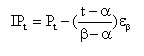
Intercensal estimates are then rounded to the nearest integer.
The residual is calculated for each month in the intercensal period. This residual is an added component that is used to balance the adjustments made to the population for the error of closure. It is calculated as follows:
For the month containing the date of the previous census of the intercensal period under consideration (m(![]() ), for example, May 2001):
), for example, May 2001):
Equation 1.4:
![]()
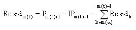
For the months m(t) between the two censuses m(![]() ) and m(β) (for example, June 2001 to April 2006):
) and m(β) (for example, June 2001 to April 2006):
Equation 1.5:
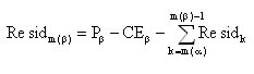
For the month containing the date of the recent census of the intercensal period under consideration (m(β), for example, May 2006):
Equation 1.6:
where
CE = censal estimates.
The sum of all these residuals should equal to the total error of closure.
1.2.2 Provincial and territorial intercensal population estimates by age and sex
The error of closure for each sex and single year of age is the difference between the census estimates (after adjustment for CNU5) and the estimated populations, calculated using the same method as is applied to the total population. The production of the intercensal estimates by age and sex involves three steps:
- the calculation of the error of closure by age and sex;
- the distribution of this error;
- a final adjustment to ensure consistency with total population figures estimated independently.
With the exception of ages between 0 and 4 years, and 100 years and over, the error of closure associated with each sex and single year of age is distributed linearly, as a function of the time elapsed since the previous census. Distributing the error of closure between censuses following specific cohorts generates intercensal estimates. Figure 1.2 shows the method for distributing the error of closure.
To calculate an intercensal estimate at time t for a given province (or territory) p, a particular age a and sex s cohort, we must first define the following:
- The dates of the two censuses ( and β).
- The date of the estimate that is required (t).
- The error of closure by province, age and sex (εp, a, s)
- The postcensal estimates of the population at time t for province p, age a and sex s (Pt(p, a, s))
- The variable n which denotes the number of whole years that separates t and β. For example, if t = 1st of July 2003 and β = 16th May 2006, then n = 2.
The following Lexis diagram (Figure 1.2) is used to illustrate a general example of the intercensal estimate by age and sex.
Figure 1.2
Lexis diagram showing intercensal estimation
Description for figure 1.2
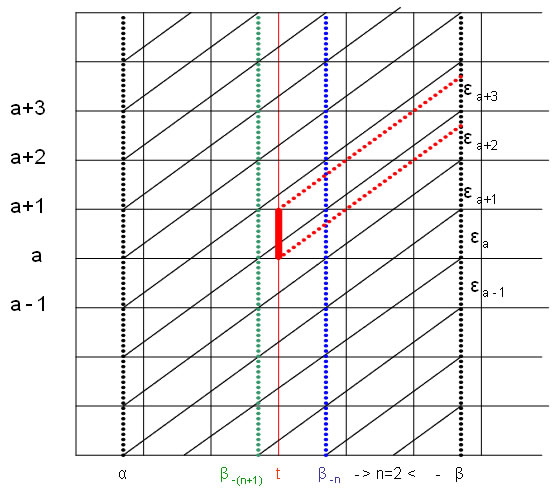
The intercensal estimate at time t for province or territory p, for age a and sex s is calculated differently based on the date and age:
A. If t-a >
![]() (meaning that the age cohort or part of the cohort was born after the previous census) the following formula is used:
(meaning that the age cohort or part of the cohort was born after the previous census) the following formula is used:
Equation 1.7:

where
ft, a, x = is the fraction of the age cohort at time t aged x (which is either a+n or a+n+1 at the time of the current census β), this is the portion of time between ![]() and t in relation to the whole intercensal period.
and t in relation to the whole intercensal period.
To calculate this fraction we use:
p = date at the start of births for this cohort;
q = date at the end of births for this cohort.
These are assigned as follows:
If X=a+n, then p= β-(a+n+1) and q=t-a
If X=a+n+1, then p= t-(a+1) and q = β-(a+n+1)
Once we have p and q, we calculate ft,a,x as follows:
Equation 1.8:
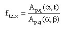
where
Ap,q(i,j) = area between time i and j of the cohort where the births have occurred between p and q.
It is noteworthy that this area is relative to the size of the cohort (q-p). These results remain valid given that the size of the cohort cancels out in the calculation of ft,a,x.
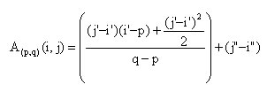
To calculate Ap,q(i,j) we need to derive the following variables:
i' = max (i, p);
j' = max(min(j,q), i );
i" = max (i, q);
j" = max(j, q);
We then calculate the area using the following formula:
Equation 1.9:
where p=q, then we set ft,a,x= 1. This is arbitrary and will not affect the outcome since the condition to have p=q implies that this term of the equation is nil.
B. If (t-a <=
![]() ) and (a <= agemax-n-2) meaning no births in the intercensal period are involved and the last age cohort is still bounded by the current census (β):
) and (a <= agemax-n-2) meaning no births in the intercensal period are involved and the last age cohort is still bounded by the current census (β):
In this case the general formula described previously can still be used. In fact we can show that if (t-a <= ![]() ) and (a <= agemax-n-2), the formula reduces to the following expression:
) and (a <= agemax-n-2), the formula reduces to the following expression:
Equation 1.10:

C. If a = agemax-n-1, the age cohorts that will age to the last unbounded age cohort during the intercensal period:
Once the age cohort reaches agemax-n-1, we have to take into account cohorts that are as old or older than the maximum age that is released in the estimates program (agemax) at the time of the recent census (β). At agemax-n-1, we use the error of closure for agemax-1 and agemax.
Equation 1.11:
In the case where  equal to the summation of P at time (t) by (p,i,s) from (i) equals to (n) to (i) equals to (agemax), we suppose a uniform distribution and the equation reduces to :
Equation 1.12:
D. If a >= agemax – n these are the remaining cohorts in the unbounded category:
In this last case, we are looking at the age cohorts that are at agemax or older at time β.
Equation 1.13:
In the case where  equal to the summation of P at time (t) by (p,i,s) from (i) equals to (agemax-n-1) to (i) equals to (agemax), we suppose a uniform distribution and the equation reduces to:
Equation 1.14:
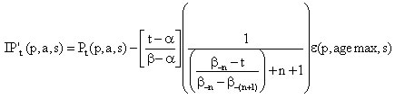
Special adjustment of the intercensal estimate to maintain coherence with the intercensal population estimated by province
Since the error of closure is estimated by cohorts, the intercensal estimates by age and sex will not exactly match the total by province as measured in the first part of this chapter. A final adjustment is done to ensure that both estimates are consistent.
Equation 1.15:
where IPttotal(p) is the intercensal estimate measured for province p using Equation 1.3 to Equation 1.6 at time t.
The special case where the intercensal population estimate becomes negative
It can happen, although rarely, that for certain age and sex cohorts for certain provinces or territories that have very low counts, are assigned a negative population count with the above mentioned methodology. In these cases, the counts will be set to zero and the difference will be redistributed proportionately in all the other cohorts. The estimates are then rounded to the nearest integer.
Notes:
- Unless otherwise noted, the adjustment for the census net undercoverage (CNU) also includes the incompletely enumerated Indian reserves.
- In addition to federal and provincial government departments, Statistics Canada also receives data files from the Office of Immigration Statistics, U.S. Department of Homeland Securitywhich is a data source to estimate emigration to the United States.
- The acronym for updated postcensal estimates is PR as this level of estimates is the revised version of the preliminary postcensal estimates.
- The acronym for final postcensal estimates is PD due to its French term postcenitaires définitives.
- The CNU by age and sex was produced by a model-based methodology as reliable estimates were not available due to insufficient sample.
- Date modified: