Explainable Machine Learning, Game Theory, and Shapley Values: A technical review

By: Soufiane Fadel, Statistics Canada

Machine learning models are often seen as an opaque black box. They take a collection of features to use as input and generate predictions. Following the training phase, a few common questions come up. How do different features influence prediction results? What are the most significant variables influencing prediction outcomes? Should I believe the findings, despite the fact that the model performance indicators seem to be excellent? As a result, model explainability is important in machine learning. The insights obtained from such interpretability methods are useful for debugging, guiding feature engineering, directing future data collection, informing human decision-making, and building trust.

To be more specific, let us distinguish between two critical ideas in machine learning – interpretability and explainability. Interpretability refers to the degree to which a machine learning model can accurately link a cause (input) with an outcome (output). On the other hand, explainability refers to the degree to which the internal workings of a machine or deep learning system can be articulated in human words. In other words, it's the ability to explain what's happening.

In this article, we'll also look at Shapley values, which are one of the most often-used model explanation methods. We'll provide a technical overview of the details underlying Shapley value analysis and outline the foundation of how Shapley values are computed by mathematically formalizing the concept and by also showing an example to illustrate the Shapley value's analysis within a machine learning problem.

What are Shapley Additive exPlanations (SHAP) values?

If you search for 'SHAP analysis' you'll discover that the word originates from a 2017 article by Lundberg and Lee, titled "A Unified Approach to Interpreting Model Predictions", which introduces the idea of "Shapley Additive exPlanations" (also known as SHAP). When using SHAP, the aim is to provide an explanation for a machine learning model's prediction by computing the contribution of each feature to the prediction. The technical explanation for the concept of SHAP is the computation Shapley values from coalitional game theory. Shapley values were named in honour of Lloyd Shapley, who introduced the concept in 1951 and went on to win the Nobel Memorial Prize in Economic Sciences in 2012. Simply put, Shapley values are a method for showing the relative impact of each feature (or variable) we're measuring on the eventual output of the machine learning model by comparing the relative effect of the inputs against the average.

Game Theory and Cooperative Game Theory

First, let's explain game theory so we can understand how it's used to analyze machine learning models. Game theory is a theoretical framework for social interactions with competing actors. It's the study of optimum decision-making by independent and competing agents in a strategic context. A "game" is any scenario in which there are many decision makers, each of whom seeks to maximize their outcomes. The optimal choice will be influenced by the decisions of others. The game determines the participants' identities, preferences, and possible tactics, as well as how these strategies influence the result. In the same context, cooperative game theory (a branch of game theory) posits that coalitions of players are the main units of decision-making and may compel cooperative conduct. As a result, cooperative games may be seen as a competition between a coalition of players rather than between individual players. So the goal is to develop a "formula" for measuring each player's contribution to the game, this formula is the Shapley value.

Shapley Values: Intuition

The scenario is as follows: a coalition of players collaborates in order to achieve a specific total benefit as a result of their collaboration. Given that certain players may make more contributions to the coalition than others and that various players may have varying levels of leverage or efficiency, what ultimate distribution of profit among players should result in any given game? In other words, we want to know how essential each participant is to the total collaboration, and what kind of reward can he or she anticipate as a result? One potential solution to this issue is provided by the Shapley coefficient values. So within the machine learning context, the feature values of a data instance serve as coalition members. Shapley values will then tell us how to divide the "payout" among the features in a fair manner, which is the prediction. A player may be a single feature value, as in tabular data. A player may alternatively be defined as a set of feature values.

Shapley Values: Formalism

It's important to understand the mathematical basis and the properties that support the Shapley value framework. This will be discussed in more detail in this section.

Shapley value formula

The Shapley value is defined as the marginal contribution of variable value to prediction across all conceivable "coalitions" or subsets of features. In other words, it is one approach to redistribute the overall profits among the players, given that they all cooperate. The amount that each "player" (or feature) gets  after a game is defined as the following:

${\varphi }_i\left(x\right)=\sum _{S\subset F\left\{i\right\}} \frac{\left|S\right|!\left(\left|F\right|-\left|S\right|-1\right)!}{\left|F\right|!}\left[f_{S\cup \left\{i\right\}}\left(x_{S\cup \left\{i\right\}}\right)-f_S\left(x_S\right)\right]$

Where:

• $x$: the observation input
• ${\varphi }_i\left(x\right)$: Shapley value for the feature $i$ for the input $x$ for the game/model $f$.
• $F$: the set of all features
• $f_S$: the trained model on the subset of features $S$.
• $f_{S\cup \left\{i\right\}}$: the trained model on the subset of features $S$ and $\left\{i\right\}$.
• $x_S$: the restricted input of $x$ given the subset of features $S$.
• $x_{S\cup \left\{i\right\}}$: the restricted input of $x$ given the subset of features $S$ and $\left\{i\right\}$.

This could be reformulated and expressed as:

${\varphi }_i\left(x\right)=\underset{\text{Averaging} }{\underbrace{\frac{1}{\left|F\right|}\sum _{S\subset F\left\{i\right\}}}}\underset{\text{combinatorial weights}}{\underbrace{{\left(\begin{array}{c}\left|F\right|-1\\ \left|S\right|\end{array}\right)}^{-1}}}\underset{\text{marginal contribution}}{\underbrace{\left[f_{S\cup \left\{i\right\}}\left(x_{S\cup \left\{i\right\}}\right)-f_S\left(x_S\right)\right]}}$

The concept of Shapley values may be split into three components: averaging, combinatorial weights, and marginal contribution. It's preferable to read from right to left while developing intuition.

• The marginal contribution is how much the model changes when a new feature $i$ is added. Given a set of features $S$, we denote $fs$ as the model trained with features $S$ present. $f_{S\cup \left\{i\right\}}$ is the model trained with an extra feature $I$. When these two models make different predictions, the quantity between square bracket is exactly how much they differ from each other.
• Combinatorial weight is the weight to give to each of the different subsets of features with size $\left|S\right|$ (excluding the feature $i$).
• And finally, averaging will determine the average of all marginal contributions from all conceivable subset sizes ranging from $0$ to $\left|F\right|- 1$. We must omit the one feature for which we wish to evaluate the feature's importance.

Theoretical Properties

Shapley values have a number of desirable characteristics; such values satisfy the following four properties: Efficiency, Symmetry, Dummy, and Linearity. These aspects may be considered a definition of a fair weight when taken together.

Four properties of a Shapley value

	Definition	Mathematical formalism
Efficiency	The sum of the Shapley values of all features equals the value of the prediction trained with all the features, so that the total prediction is distributed among the features.	$\begin{array}{l}\sum \end{array}_{\begin{array}{l}i\in F\end{array}}{\varphi }_i\left(x\right)=f_F\left(x\right)$
Symmetry	The contributions of two feature values should be the same if they contribute equally to all possible coalitions.	$\begin{array}{c}[\forall S\subset F\backslash \{i,j\}:f_{S\cup \left\{i\right\}}\left(x_{S\cup \left\{i\right\}}\right)=f_{S\cup \left\{j\right\}}\left(x_{S\cup \left\{j\right\}}\right)]\\ \Downarrow \\ {\varphi }_i\left(x\right)={\varphi }_j\left(x\right)\end{array}$
Dummy	A feature that does not change the predicted value regardless of which coalition of feature values it is added to should have a Shapley value of $0$.	$\forall S\subset F:\left[f_{S\cup \left\{i\right\}}\right(x_{S\cup \left\{i\right\}})=f_S(x_S)\Rightarrow {\varphi }_i(x)=0]$
Linearity	If two models described by the prediction functions $f$ and $g$ are combined, the distributed prediction should correspond to the contributions derived from $f$ and the contributions derived from $g$.	${\varphi }_i^{f+g}\left(x\right)={\varphi }_i^f\left(x\right)+{\varphi }_i^g\left(x\right)$ $\forall a\in R {\varphi }_i^{a.f}\left(x\right)=a.{\varphi }_i^f\left(x\right)$

Consider the following scenario: You trained a random forest model, which implies the prediction is based on an average of several different decision trees. You may compute the Shapley value for each tree independently, average them, and use the resulting Shapley value to calculate the feature value in a random forest. This is guaranteed by the linearity property.

Machine Learning Application Example: Interpretability

The theoretical qualities of Shapley values are all interesting and desirable to have, but in practice we may not be able to determine the precise Shapley value because of practical constraints. Obtaining the precise Shapley value formulation takes a significant amount of processing time. When it comes to real-world situations, the approximate answer is often most practical because there are $2^{\left|F\right|}$ potential coalitions of the feature values. Calculation of the exact Shapley value is computationally too costly. Fortunately, we can apply certain approximation approaches; the quality of these techniques affects how well the theoretical characteristics hold. Several research tests have been conducted to demonstrate the SHAP approximation results are more consistent when compared to the values produced by other commonly used algorithms.

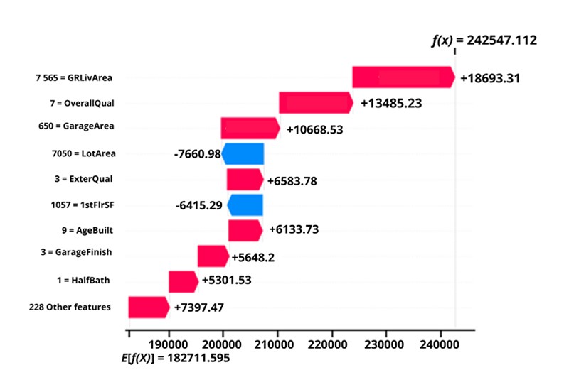
The following figure will provide an example of how to examine the contributions of features to investigate the predictions of an "Xgboost" model that estimates the sale price for homes using 237 explanatory variables, describing nearly every aspect of residential homes in Ames, lowa. The dataset for this analysis is publicly accessible on: Kaggle - House Prices - Advanced Regression Techniques.

Figure 1

The bottom of this plot starts as the expected value of the model output (182K). Each row above it, shows how the positive (red) or negative (blue) contribution of each feature moves the value from the expected model output, to the model output for this prediction (242K). The gray text before the feature names shows the value of each feature for this sample. According to this graph, we can conclude that 228 other features add a total of $7,397.47 to the predetermined value. And that each numbered variable above impacts the value by over $5,000. The expected price of this particular home climbs to over $18,000 with a floor area of 7,500 square feet. The price is discounted by $7,660.98 due to the size of the lot being 7,050 square feet.

Conclusion

As discussed, Shapley values have mathematically satisfied theoretical properties as a solution to game theory problems. The framework provides contrastive explanations which means that instead of comparing a prediction to the average prediction of the full dataset, you may compare it to a subset or even a single data point. It explains a prediction as a game played by the feature values.

Furthermore, this methodology is one of the few explanation methods with a strong theory, since the mathematical axioms (efficiency, symmetry, dummy, additivity) provide a reasonable foundation for the explanation.

Finally, it's worth mentioning that this strategy is only one of many possible solutions. However, the Shapley value is often preferable since it is based on a solid theory, fairly divides the effects, and provides a complete explanation.

References

Bosa, K. (2021). Responsible use of machine learning at Statistics Canada.

Cock, D. D. (2011). Ames, Iowa: Alternative to the Boston Housing Data. Journal of Statistics Education.

Molnar, C. (2021). Interpretable Machine Learning: A Guide for Making Black Box Models Explainable.

Scott Lundberg, S.-I. L. (2017). A Unified Approach to Interpreting Model Predictions.

Yadvinder Bhuller, H. C., & O'Rourke, K. (n.d.). From Exploring to Building Accurate Interpretable Machine Learning Models for Decision-Making: Think Simple, not Complex.