
Extracting Temporal Trends from Satellite Images
By: Kenneth Chu, Statistics Canada
The Data Science Division of Statistics Canada recently completed a number of research projects to evaluate the effectiveness of a statistical technique called functional principal component analysis (FPCA) as a feature engineering method in order to extract temporal trends from Synthetic Aperture Radar (SAR) satellite time series data.
These projects were conducted in collaboration with the Agriculture Division and the Energy and Environment Statistics Division of Statistics Canada, as well as the National Wildlife Research Centre (NWRC) of Environment and Climate Change Canada. These projects used Sentinel-1 data. Sentinel-1 is a radar satellite constellation of the European Space Agency’s Copernicus program. It collects SAR imagery data that captures information about Earth’s surface structures of the imaged area. Sentinel-1 provides global year-round coverage under all weather conditions of the imaged area. The data are unaffected by day and night, have high spatial resolution (approximately 10m x 10m) and a fixed data capture frequency of one data captured every 12 days, for each imaged area. Consequently, Sentinel-1 data are highly suitable for scientific studies as the Earth’s surface structures hold important information.
Our results suggest that FPCA could be a very effective tool to numerically extract seasonal temporal trends captured in a Sentinel-1 image time series, in a large-scale and high-granular fashion. This article gives a summary of the FPCA-based method and its feature extraction results from Sentinel-1 seasonal time series data.
Motivation
I will focus on one of the study areas of research, namely the Bay of Quinte area in Ontario, located near Belleville. The objective of this project is to give a more accurate wetland classification. The following is an optical satellite image (rather than a radar satellite image) of the Bay of Quinte area, downloaded from Google Maps.
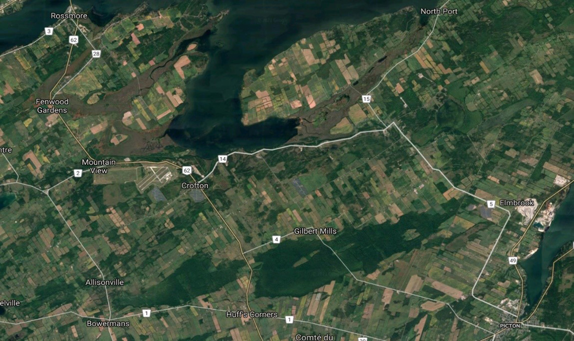
Figure 1: Optimal satellite image of Bay of Quinte, Ontario. Downloaded from Google Maps.
Description - Figure 1
Optimal satellite image of Bay of Quinte, Ontario, located in the center at the top of the image. The rest shows a generally rural sprawl of the surrounding area and includes several townships and the highways that connect them. The townships pictured include (clockwise from the top left): Rossmore, Fenwood Gardens, Mountain View, Crofton, Elmbrook, Picton, Gilbert Mills, Huff’s Corners, Bowermans and Allisonville.
In Figure 1, note the large body of water at the top-centre of the image and the rectangular agricultural fields. Also note the island near the top-centre and the waterway that separates it from the mainland.
Next, examine Figure 2, which is a land cover map of the Bay of Quinte area.
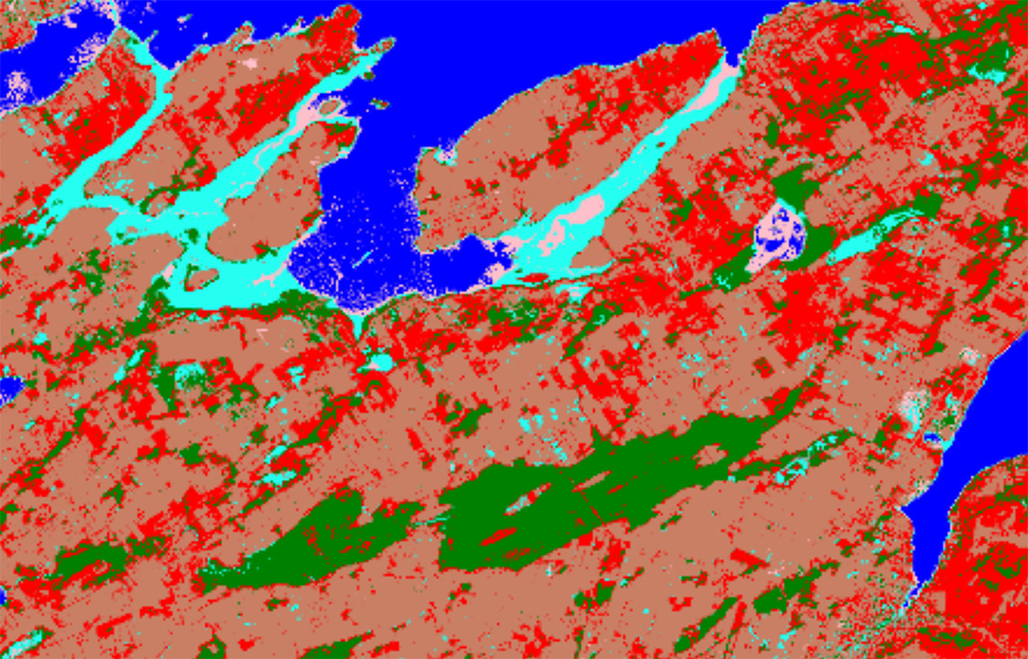
Figure 2: Land cover map of Bay of Quinte, ON. This image is created from 2019 RADARSAT-2 time series data (Banks et al., 2019). The colours indicate different land cover types: Blue indicates water, pink indicates shallow water, cyan shows marsh, red indicates forest, green is for swamp area and brown indicates agricultural land.
Description - Figure 2
Land cover map of Bay of Quinte, ON, from 2019 RADARSAT-2 time series data. The colours indicate different land cover types. The Bay of Quinte is blue, indicating water and is mostly at the top centre of the image. The outline of the Bay of Quinte is in Cyan, which denotes marsh area, and includes a few pink spots within it, indicating shallow water. The surrounding land area is mainly red, which denotes forest area, and two semi large spots in the lower centre of the image are green, highlighting a swamp area.
Figure 3 is a red, green, blue (RGB) rendering of the first three functional principal component (FPC) scores computed from 2019 Sentinel-1 time series data for the Bay of Quinte area. Note the remarkable granularity and the high-concordance level with the land cover map in Figure 2.
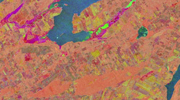
Figure 3: RGB rendering of the first three FPC scores computed from 2019 Sentinel-1 time series data for the Bay of Quinte area.
Description - Figure 3
Land cover map of Bay of Quinte. The colours indicate different land cover types. The Bay of Quinte is blue, indicating water. The outline of the Bay of Quinte is pink, and the surrounding land area is mainly orange. This image is similar to the rendering from Figure 2.
The land cover map in Figure 2 was created from RADARSAT-2 (one of Canadian Space Agency’s SAR Earth Observation satellites) time series data from 2019, using the methodology described in Banks et al. (2019). It’s well corroborated with ground truth collected via field observations. A notable observation here is that the waterway separating the island in the top-centre of the image and the mainland, in fact contains two types of wetland – marsh in cyan and shallow water in pink. These two wetland types are not easily distinguishable in Figure 1. The article reported that SAR seasonal time series data contain sufficient information f or wetland classification, but the methodology described involved a high degree of manual decision-making informed by expert knowledge (e.g., data captures for which dates or statistics to use, etc.). It was labour-intensive and it wasn’t clear on how to automate that methodology and scale it to a regional, provincial or pan-Canada scale.
The motivation behind the Bay of Quinte project was to seek an automatable and effective methodology for numerically extracting temporal trends from seasonal SAR time series data in order to facilitate downstream land cover classification tasks.
Main results: Visualization of FPCA-based extracted features
FPCA has the potential to be a powerful methodology for extracting dominant trends from a collection of time series (Wang et al. 2016). Therefore, we carried out a feasibility study on the use of FPCA as a feature extraction technique for the pixel-level SAR seasonal time series data. The resulting features are FPC scores, at the pixel-level. Our preliminary results suggest that the FPCA-based methodology could be remarkably effective. Figure 3 is the RGB rendering of the first three FPC scores (first FPC score is the red channel, second FPC score is green, third FPC score is blue (Wikipedia 2022); computed from the 2019 Sentinel-1 time series data for Bay of Quinte. Note the remarkable granularity of Figure 3 and its high level of concordance with Figure 2. This strongly suggests that these FPCA-based extracted features may significantly facilitate downstream land cover classification tasks. The rest of this article will explain how Figure 3 was generated from Sentinel-1 time series data.
Overview of FPCA-based feature extraction procedure
A quick overview of the procedure is as follows:
- A subset of locations/pixels were carefully and strategically selected from the Bay of Quinte study area.
- Their respective Sentinel-1 time series were used to train an FPCA-based feature extraction engine.
- The trained FPCA-based feature extraction engine was then applied to the Sentinel-1 time series of each location/pixel of the entire Bay of Quinte area. The output of each time series is an ordered sequence of numbers called FPC scores for the corresponding location/pixel. The order of these scores is in descending order of variability explained by their corresponding FPC.
- Figure 3 above is the RGB rendering of the first three FPC scores of the 2019 Sentinel-1 time series data.
The training data
The collection of training data (from the locations/pixels from the Bay of Quinte area) were carefully and strategically chosen to contain specific properties.
- The training locations were distributed throughout the Bay of Quinte study area.
- The land cover types were known based on prior field observations.
- There were six land cover types represented in the training collection: water, shallow water, marsh, swamp, forest, and agriculture land.
- The training collection were well-balanced across land cover types as each land cover type contained exactly 1000 locations/pixels (except for shallow water, which had 518).
- The six land cover types represented in the training collection are comprehensive as every location/pixel in the Bay of Quinte study area are covered by one of these six land cover types.
The Sentinel-1 data have two polarizations – vertical transmit and vertical receive (VV), and vertical transmit and horizontal receive (VH). These two polarizations can be regarded as two observed variables measured by the Sentinel-1 satellites.
Different Earth surface structures are detected with different sensitivities in polarizations. For example, rough surface scattering, such as those caused by bare soil or water, is most easily detected in the VV polarization. On the other hand, volume scattering, commonly caused by leaves and branches in a forest canopy, is most easily detected in VH and HV polarizations. Finally, a type of scattering called double bounce, commonly caused by buildings, tree trunks, or inundated vegetation, is most easily detected in the HH polarization (NASA 2022). For the rest of this article, we will focus on VV polarization.
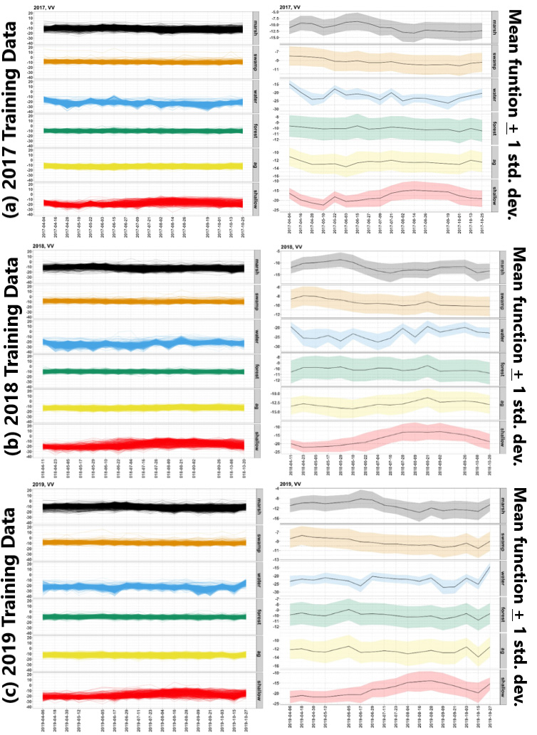
Figure 4: Sentinel-1 VV time series data of the training locations and corresponding ribbon plots for easy temporal trend visualization. (a): 2017 data. Left panel group: Line plots of the Sentinel-1 VV time series data grouped by known land cover types. Right panel group: Corresponding ribbon plots, with the black curve in each panel indicating the panel-specific mean curve, and the ribbon indicating one standard deviation above and below the panel-specific mean curve. (b), (c): 2018, 2019 data, respectively.
Description - Figure 4
Each panel corresponds to one of the six wetland types for 2017, 2018 and 2019 – marsh, swamp, water, forest, agriculture and shallow water. Each panel contains 1000 training time series, corresponding to 1000 distinct training locations, except for the bottom panel, which has only 518 time series. The horizontal axis shows the observation dates. They are 12 days apart, except the occasional gaps. The following four points are observed for the 2017, 2018 and 2019 time series data:
- Observation 1: The collection of observation dates can change from year to year, and so can the gaps.
- Observation 2: Water and Shallow water on average have lower values than the rest of the wetland types.
- Observation 3: From the Shallow Water ribbon plot, one sees that Shallow Water shows a distinct trend, starting low early in the growing season and then peaking in late August.
- Observation 4: From the Marsh ribbon plot, one sees that Marsh exhibits roughly the opposite trend as the Shallow Water, namely starting high and then coming down later in the season.
Functional principal component analysis
We give a conceptual explanation of FPCA via a comparison to the familiar ordinary principal component analysis (OPCA).
The OPCA is:
- Suppose a finite set (of data points) is given.
- Find orthogonal directions, more precisely, one-dimensional subspaces in along which exhibits the most variability, the second most, the third most, and so on. Here, orthogonality is defined via the standard inner product (dot product) on . For each orthogonal one-dimensional subspace, choose a unit vector within that subspace. The resulting mutually orthogonal unit vectors are the ordinary principal components, and they form an orthonormal basis for .
- Rewrite each , in terms of the ordinary principal components. The coefficients of this linear combination are the ordinary principal component scores of with respect to the ordinary principal components.
How does FPCA (more precisely, the particular flavour of FPCA we used) differ from OPCA ?
- The finite-dimensional vector space is replaced with a (possibly infinite-dimensional) sub-space of the -integrable functions defined on a certain (time) interval .
- The standard inner product on is replaced with the inner product on F, i.e., for ,
Why can FPCA capture temporal trends ?
- This is because the “geometry” of the interval is incorporated in the very definition of the inner product. More concretely put, the integration process of functions over incorporates information about the ordering and distance between every pair of time points.
- This “awareness” of the geometry of the interval in turn allows the inner product to capture information about temporal trends.
General procedure to apply FPCA to time series data
- Suppose a finite set of observed time series is defined on a common set of time points within a certain time interval (e.g., within the growing season of a certain calendar year), where and are respectively the initial and final common timepoints.
- Interpolate each given time series in to obtain a function defined on . This yields a finite set of functions defined on the common interval , each of which is an interpolation of one of the original observed time series in .
Note: B-splines are a common choice of interpolation techniques for this purpose (Schumaker, 2022). - Compute the global mean function and an ordered sequence of functional principal components for the collection of functions (interpolations of time series in as a whole. Note that each FPC is itself a function defined on 2016).
Then, for each function in , express it as a linear combination of the FPC. The coefficients of this linear combination are the FPC scores of the given function with respect to the FPC.
Consequently, the functions in , the FPC, and the FPC scores can be organized as follows:
As more FPCs are included, the approximations above should increase in accuracy.
- We consider the global mean function and the ordered sequence of FPCs to be what has been learned from the functions in using the FPCA machinery.
- Lastly, note that once the global mean function and the FPCs of have been computed ( or “learned”), they can be used to compute scores for new functions defined on , in particular for interpolations of new time series. It is this observation that enables the FPCA machinery to be used as a feature engineering technique.
FPCA-based feature extraction workflow
We explain how the FPC scores that underlie Figure 3 were computed in the Bay of Quinte project.
- As described earlier, a collection of “training” locations/pixels from the Bay of Quinte study area were meticulously chosen, as described earlier.
- The 2017, 2018, 2019 Sentinel-1 time series data were extracted for each training location/pixel in . We denote the resulting collection of time series by .
- Each time series in was interpolated using B-splines. We denote the resulting collection of functions by .
- The global mean function and the set of functional principal components were computed (“learned”) from using the FPCA machinery. This FPCA machinery has been implemented in the form of the R package fpcFeatures (currently, only for internal use at NWRC and Statistics Canada).
- The 2017 Sentinel-1 time series for each of the non-training location/pixel from the Bay of Quinte study area was interpolated with B-splines. For each of the resulting B-spline interpolations, the FPC scores with respect to the learned functional principal components were computed. Similarly for the 2018 and 2019 non-training Sentinel-1 time series.
- The resulting FPC scores are regarded as the extracted features for each location/pixel. These extracted features may be used for downstream analytical or processing tasks, such as visualization (such as RGB rendering), land cover classification, land use change detection, etc.
This FPCA-based feature extraction workflow is illustrated in Figure 5.
Figure 5: Schematic of FPCA-based feature extraction workflow.
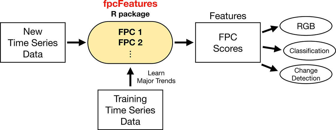
Description - Figure 5
FPC Features diagram begins with a square for New Time Series Data that feeds into the R package, which contains FPC 1, FPC 2, etc. A square for Training Time Series Data also feeds up to the R package. From there, the R package points to the next step which is are the Features or FPC Score. And from there extracted features are generated, which can be used in downstream processing or analytical tasks, e.g., visualization via RGB rendering, land use classification, land use change Detection.
The computed functional principal components
If you recall, the so-called “trained FPCA-based feature extraction engine” is really just the global mean function and the ordered sequence of FPCs (functions defined on a common time interval) computed from the training data. Figure 6 displays the first seven FPCs computed from the 2017, 2018 and 2019 training Sentinel-1 VV time series data from the Bay of Quinte study area.
Figure 6: Graphical representations of the first seven functional principal components as functions of time.
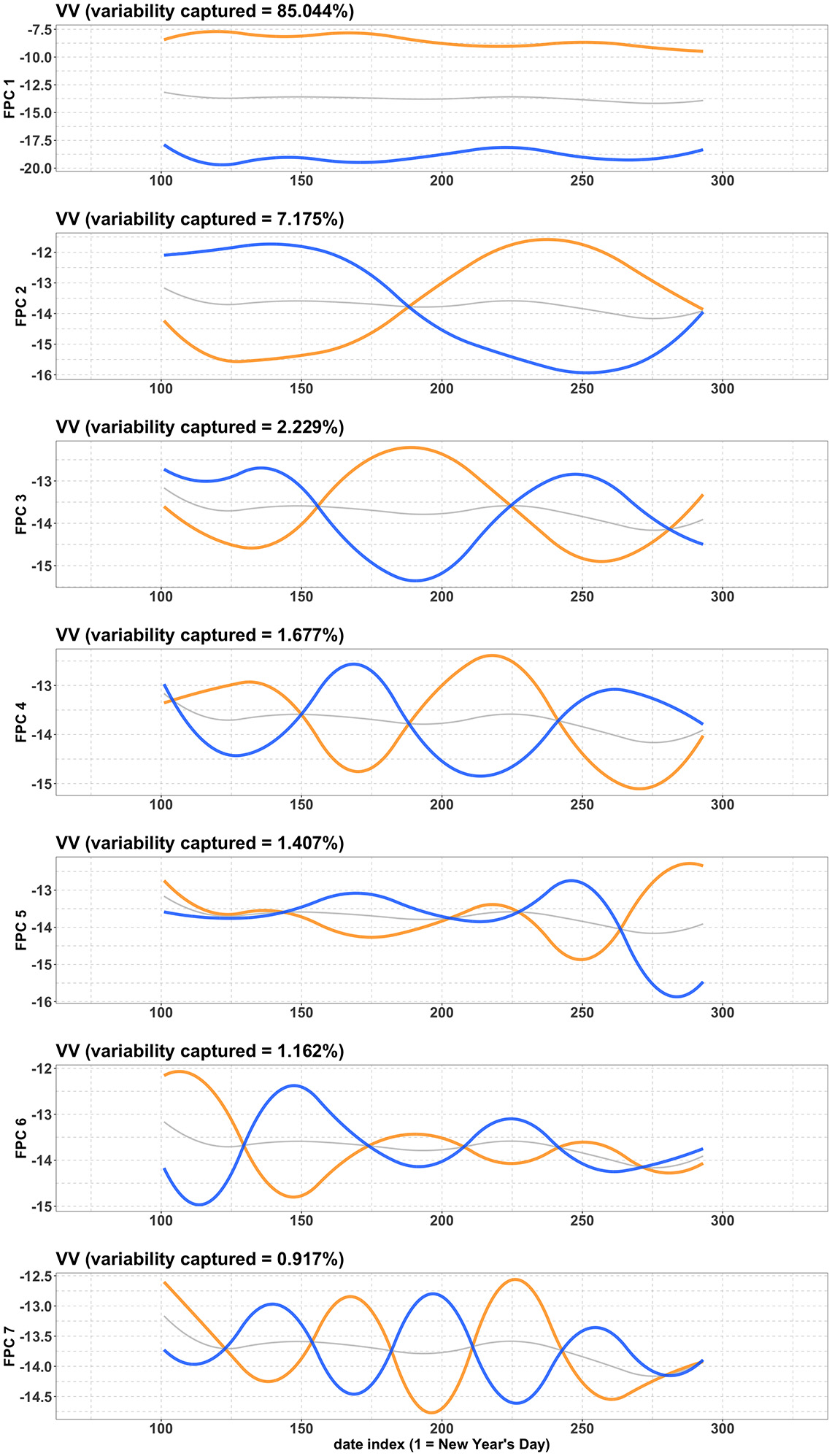
Description - Figure 6
Seven FPC line graphs computed from the 2017, 2018 and 2019 training Sentinel-1 time series data. In each panel, the horizontal axis represents the “date index,” where 1 refers to New Year’s Day, 2 refers to January 2, and so on. The vertical axis represents the value of the respective FPC scores. FPC 1 – Variability captured = 85.044%; FPC 2 – Variability captured = 7.175%; FPC 3 – Variability captured = 2.229%; FPC 4 – Variability captured = 1.677%; FPC 5 – Variability captured = 1.407%; FPC 6 – Variability captured = 1.162%; FPC 7 – Variability captured = 0.917%. A further explanation is below.
These are graphical representations of the first seven FPCs as functions of time. The (counting from top) panel visualizes the FPC. Recall that each FPC is, first and foremost, a (continuous) function of time, viewed as a vector in a certain vector space of (-integrable) functions defined on a certain time interval.
In each panel, the grey curve indicates the mean curve of the spline interpolations of all the VV time series (across all training locations and across years 2017, 2018 and 2019). The FPC turn out to be eigen vectors of a certain linear map (related to the “vari ance” of the training data set) from to itself (Wang et al. 2016). In each panel, the orange curve is the function obtained by adding to the mean curve (in gray) the scalar multiple of the functional principal component , where is the eigenvalue corresponding to . The blue curve is obtained by subtracting the same multiple of from the mean curve. Note as well that the first principal component explains about 85.04% of the variability in the training data (VV time series), the second component explains about 7.18%, and so on.
Next, note that the first functional principal component resembles a horizontal line (orange curve in top panel); it captures the most dominant feature in the training time series, which turns out to be the large near-constant difference in VV values between the Water/Shallow Water time series and those of the rest of the (non-water) land cover types. This large near-constant difference is clearly observable in the line and ribbon plots in Figures 4, 5, and 6.
Lastly, note that the second functional principal component (orange curve in second panel) has an early-season trough and a late-season peak, which captures the Shallow Water trend, as observable in the Shallow Water ribbon plots in Figures 4, 5, and 6.
The first two FPC scores of the training data
We show here the scatter plots of the first FPC score against the second for the training data. Note the well separation of the water and shallow water training locations from those of the other land cover types, and note the consistency across years of this well separation.
Figure 7: 2017 FPC scores – training
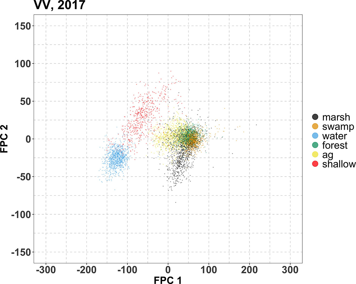
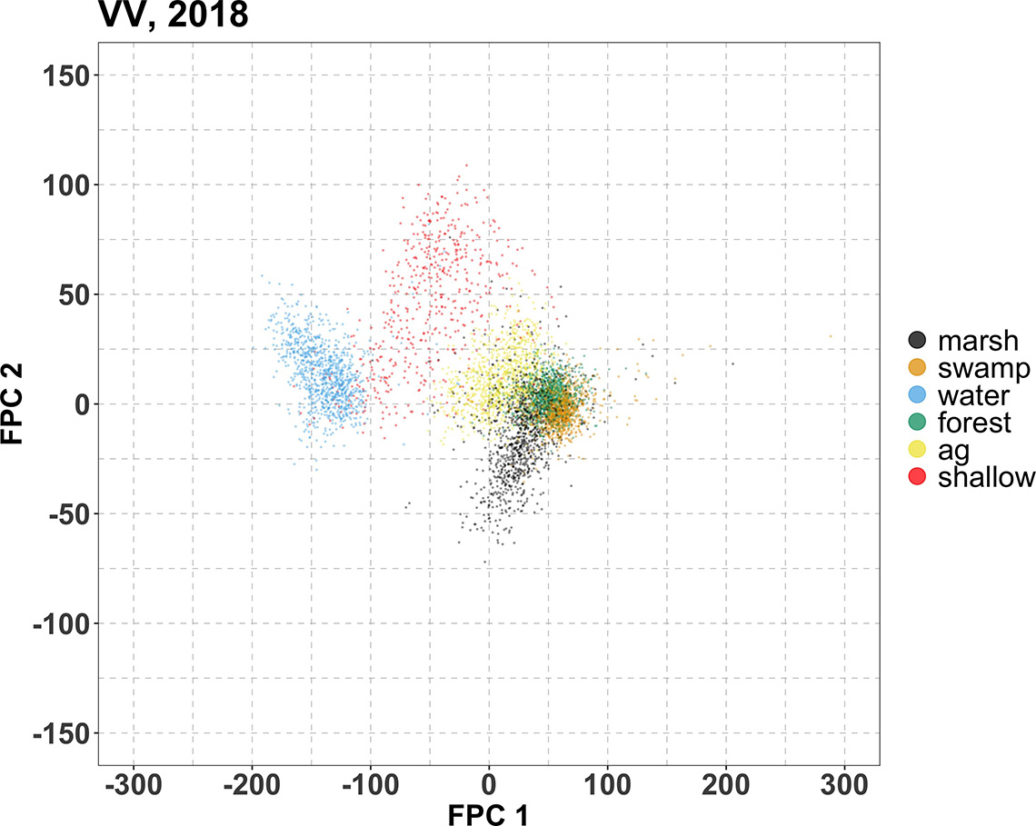
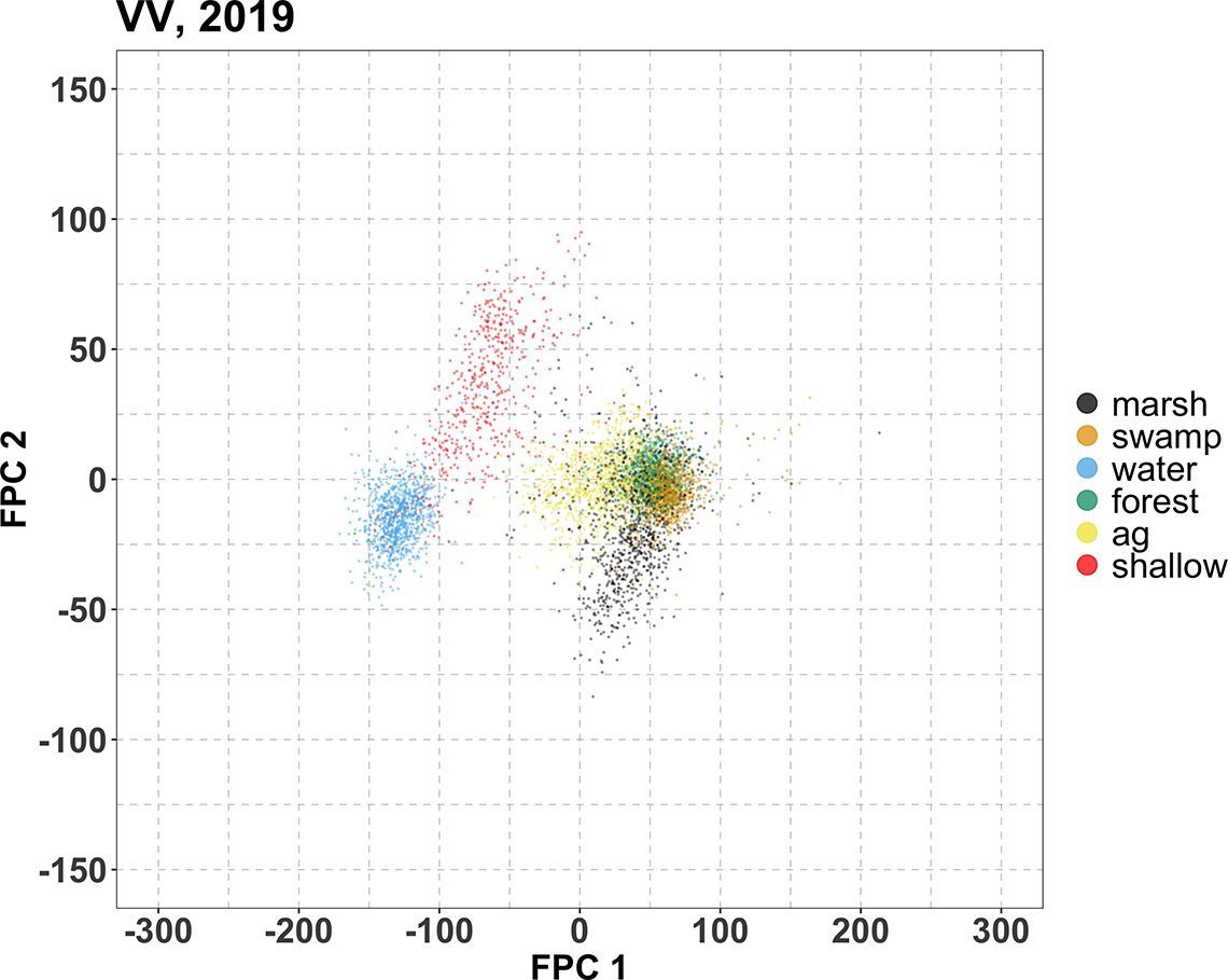
Description - Figure 7
Scatter plots of the first FPC score against the second for the 2017, 2018 and 2019 training time series data. The FPC scores are regarded as the extracted features. Each data point in this plot corresponds to a training location, with its colour indicating its wetland type. The horizontal and vertical axes correspond respectively to the first and second FPC scores derived from the VV time series. We emphasize that, while each plot shows only the scores of their corresponding training time series year, the FPC scores were computed simultaneously for all VV time series across all years and all wetland types.
The data points are partially clustered by wetland type; in particular, the water and shallow water separate very well from the rest of the wetland types. The horizontal (which is the dimension corresponding to the first FPC) separation between water/shallow water from the rest. This is a manifestation of the large vertical difference between water/shallow water and the rest of the non-water wetland types in terms of the original VV values (refer to figures 4). The first FPC captures this large vertical difference consistent throughout the growing season, and this explains why the first FPC resembles a flat line (orange curve that would appear in the top panel of Figure 6).
Also recalling that the second FPC has a trend that resembles that of the shallow water (as noted in the ribbon plots in the bottom panels of figure 4 against the orange curve in the second panel in Figure 6). Recall also that the marsh roughly exhibits the opposite trend (as noted in the top panel of figures 4 against the blue curve in the second panel in Figure 6). The second FPC captures the trend exhibited by shallow water, and accordingly, in this scatter plot is the shallow water training locations (red) that extend significantly in the positive vertical direction. Conversely, since the marsh exhibits roughly the opposite trend, the marsh training locations (black) extend significantly downward in the present scatter plot.
Sanity check: approximation of original training time series via FPCA
Given that the FPCA hinges on approximating individual training data time series as linear combinations of a sequence of FPCs (themselves functions) that are learned from the training data time series as a group:
To assess the suitability of FPCA to a specific given time series data set, it is prudent to examine how well the FPCA-based approximations can actually approximate the original given time series data.
Figure 12 displays six randomly chosen Sentinel-1 training data time series and their FPCA approximations to give an impression of the goodness-of-fit of the FPCA approximations.
Figure 8: FPCA approximations of six training data time series.
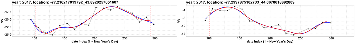
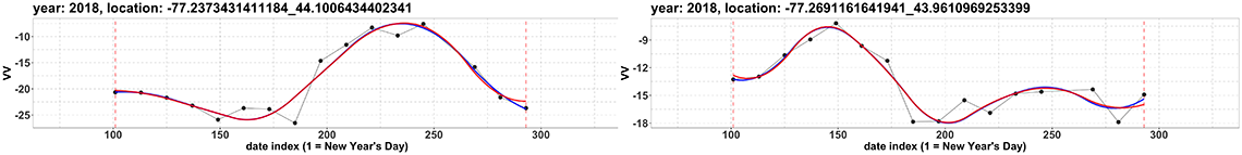
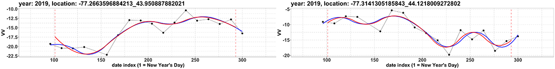
Description - Figure 8
FPCA approximations of six training data time series. In each panel, the horizontal axis represents the “date index,” where 1 refers to New Year’s Day, 2 refers to January 2, and so on. The vertical axis represents the value of the VV variable in the Sentinel-1 data. The black dots are the original time series data points. The blue curve is the B-spline interpolation. The red curve is the seven-term FPCA approximation of the B-spline interpolation (blue curve), where “seven-term” here means that the FPCA approximation is the sum of the global mean function and a linear combination. Panel 1 – year 2017, location: -77.210217019792_43.8920257051607; Panel 2 – year 2017, location: -77.2997875102733_44.0678018892809; Panel 3 – year 2018, location: -77.2373431411184_44.1006434402341; Panel 4 – year 2018, location: -77.2691161641941_43.9610969253399; Panel 5 – year 2019, location: -77.2663596884513_43.950887882021; Panel 6 – year 2019, location: -77.3141305185843_44.1218009272802
Future work
- This article showcases the FPCA-based feature engineering technique for seasonal Sentinel- 1 time series data. Recall however, that the ultimate goal is classification of wetland. The immediate follow-up research is to apply some “basic” (e.g., random forest) classification techniques to the FPCA-based extracted features (i.e., FPC scores) and examine the resulting accuracies.
- Most basic classification techniques such as the random forest, would ignore the spatial relationships among the locations/pixels. If the basic techniques turn out to yield insufficient accuracies, you consider more sophisticated classification techniques that attempt to take into account the spatial relationships, e.g., by essentially imposing constraints that favour nearby locations/pixels to have the same predicted land cover type. One such technique is the hidden Markov random field, treating the land cover classification task as an unsupervised image segmentation problem.
- Figure 3 took approximately 45 minutes to generate, running in 16 parallel threads on a single x86 64-conda-linux-gnu (64-bit) virtual computer, on a commercial computing cloud, with 28 GB of memory, using the Ubuntu 20.04.2 LTS operating system, and R version 4.0.3 (2020- 10-10). However, Figure 3 covers only the Bay of Quinte study area, which is a tiny area compared to the province of Ontario, or to all of Canada. Using the same computing resources mentioned above to execute the FPCA-based feature extraction workflow would require about three weeks for Ontario, and several months for all of Canada. Several years’ worth of Sentinel- 1 data for all of Canada will have a storage footprint of dozens of terabytes. On the other hand, ultimately, one would indeed like to implement a (nearly fully) automated pan-Canada wetland classification system. Distributed computing (cloud computing or high-performance computing clusters) will be necessary to deploy such a workflow that can process such volumes of data within in a reasonable amount of time. A follow-up study is well underway to deploy this workflow on Google Cloud Platform (GCP) for all of British Columbia. We expect the execution time of the GCP deployment for all of British Columbia, divided into hundreds of simultaneous computing jobs, to be under 3 hours. In addition, we mention that, due to the vectorial nature of the FPCA calculations, a GPU implementation should in theory be feasible, which could further speed up the computations dramatically. A scientific article on the results and methodologies of this series of projects is in preparation and will be published in a peer-reviewed journal shortly.
- As mentioned, seasonal changes in Earth surface structures, captured as temporal trends in Sentinel-1 time series data, are useful predictor variables for wetland classification. However, in order to use the data correctly and in a large scale, one must be cognizant of a number of potential issues. For example, data users must be well-informed of measurement artifacts that might be present in such data, how to detect their presence, and how to correct for them, if necessary. We also anticipate that temporal trends do vary (e.g., due to natural variations, climate cycles, climate change), both across years and across space. It remains an open research question as to how to take into account the spatiotemporal variations of Sentinel-1 time trends, when we design and implement a pan-Canada workflow.
- Recall that we focused exclusively on the VV polarization in the Sentinel- 1 data, though we already mentioned that Sentinel-1 data have one more polarization, namely VH. Different polarizations are sensitive to different types of ground-level structures (NASA 2022). In addition, Sentinel-1 is a C-band SAR (i.e., radar signal frequency at about 5.4 GHz) satellite constellation, which in particular implies that Sentinel-1 measures, very roughly, ground-level structures of size of about 5.5cm. However, there are other SAR satellites that have different signal frequencies, which therefore target ground-level structures of different sizes (NASA 2022). It will be very interesting to examine whether SAR data with different signal frequencies, and measured in different polarizations, could be combined in order to significantly enhance the utility of these data.
References
- BANKS, S., WHITE, L., BEHNAMIAN, A., CHEN, Z., MONTPETIT, B., BRISCO, B., PASHER, J., AND DUFFE, J. Wetland classification with multi-angle/temporal sar using random forests. Remote Sensing 11, 6 (2019).
- EUROPEAN SPACE AGENCY. Sentinel-1 Polarimetry. https://sentinel.esa.int/web/sentinel/user-guides/sentinel-1-sar/product-overview/polarimetry. Accessed: 2022-02-10.
- NASA. What is Synthetic Aperture Radar? https://earthdata.nasa.gov/learn/ backgrounders/what-is-sar. Accessed: 2022-02-10.
- SCHUMAKER, L. Spline Functions: Basic Theory, third ed. Cambridge Mathematical Library. Cambridge Mathematical Library, 2007.
- WANG, J.-L., CHIOU, J.-M., AND MU¨LLER, H.-G. Functional data analysis. Annual Review of Statistics and Its Application 3, 1 (2016), 257–295.
- WIKIPEDIA. RGB color model. https://en.wikipedia.org/wiki/RGB_color_model. Accessed: 2022-02-10.
All machine learning projects at Statistics Canada are developed under the agency's Framework for Responsible Machine Learning Processes that provides guidance and practical advice on how to responsibly develop automated processes.

If you have any questions about this article or would like to discuss this further, we invite you to our new Meet the Data Scientist presentation series where the author will be presenting this topic to DSN readers and members.
Wednesday, September 14
2:00 to 3:00 p.m. EDT
MS Teams – link will be provided to the registrants by email
Register for the Data Science Network's Meet the Data Scientist Presentation. We hope to see you there!
- Date modified: