
Image Segmentation in Medical Imaging
By: Loïc Muhirwa, Statistics Canada
Introduction
Many applications require substructures of digital images to be identified, making segmentation a fundamental preprocessing procedure. A canonical example of image segmentation is the binary segmentation between the foreground and background of an image, which is broadly applicable. In medical imaging, one might need to segment magnetic resonance (MR) or computerized tomography (CT) images of an organ into distinct anatomical structures or segment different tissue types. In neuroimaging in particular, one could segment the human brain into major tissue (white and gray matter) or segment between the health status of a tissue i.e. healthy and lesioned.
To formalize these ideas, we need a mathematical representation of an image. There are many ways to represent images, depending on the applications, some are more convenient than others. This article will present many approaches to image segmentation which makes a single mathematical representation of an image difficult. Despite this, we'll adopt a primary representation, which we may deviate from for notational convenience or to complete cases where an image is a discrete object, as opposed to a continuous one. Formally, an image can be represented as a pixel-wise map from some image domain to an intensity domain, as follows:
where the image domain is a compact space and a simply connected subset of for 2D or 3D images, also known as volumes (see: simply connected definition). Moreover, without loss of generality, this article only considers images with unidimensional intensity values, such as grayscale images. This is an implied definition since the image maps to . Under this image representation, we can conceptually specify a segmentation Z of the image I as the following map:
where is the number of distinct image segments.
Figure 1: A segmentation of an axial brain slice. Red, green and blue correspond to white matter, gray matter and cerebrospinal fluid respectively. (Image source: A review of medical image segmentation: methods and available software.Footnote 21)
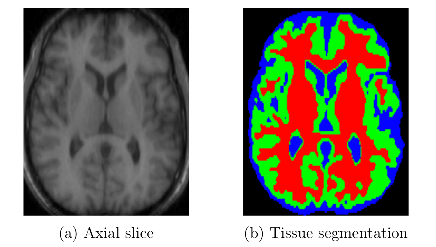
Description - Figure 1: A segmentation of an axial brain slice. Red, green and blue correspond to white matter, gray matter and cerebrospinal fluid respectively.
Brain imaging of an axial slice on the left in black and white, and tissue segmentation represented by red, green and blue on the right. Colours from the image on the right correspond to white matter, gray matter and cerebrospinal fluid respectively, from the image on the left.
Digital image segmentation can be broadly classified into two categories, manual segmentation and automated segmentation. In manual segmentation, a human manually annotates the different segments in a digital image, whereas in automated segmentation an automated algorithm segments the image. Manual segmentation comes with various challenges, including cost, time and consistency. First, in many applications, the person annotating the images needs to be a domain expert—making manual segmentation operationally challenging and costly.
In medical neuroimaging, for instance, some of the common segmentation types are tissue type segmentation, where brain tissue is categorized into three major tissue types – white matter, gray matter and cerebrospinal fluid (see figure 1). Manual annotation for a single patient's neuroimage volume requires a lot of time and radiologist knowledge. Second, image processing might require annotating hundreds of images, which is unmanageable when done manually. Third, manual segmentations vary greatly across annotators, even when the annotators are domain expertsFootnote 1. Certain scanners can produce images that could be automatically segmented with ease. For example, a CT neuroimage has intensities with fixed physical correspondence, making automated segmentation a straightforward task. For these reasons and more, automated segmentation is preferred.
In the following sections, we'll categorize automated segmentation methods into two categories – generative model-based methods and deep learning methods.
Automated Segmentation - Generative Model-Based Methods
In generative model-based methods, the segmentation of an image is modeled as a statistical inference problem. Specifically, a generative model of the image is specified, in which the segmentation is a latent variable and segmenting an image corresponds to inferring this variable.
Univariate Models
In a point-wise fashion, univariate method models image intensities from different segments as sub-populations from a finite mixture model (FMM) with different intensity distributions describing the data generating processes of different segments. Under this modelling approach image intensities belonging to specific segments are drawn from distinct mixtures. A special case of FMM that's often used in image segmentation is a Gaussian mixture model (GMM) where the mixture distributions are Gaussians.Footnote 2Footnote 3Footnote 4 We'll use a GMM to demonstrate how a generative model can be used to segment an image. The image is represented by a random variable which is a collection of independent random variables with support and let be random variable with support representing the intensity value and mixture assignment for some image domain element respectively. Let be a random variable vector with support as mixture probabilities, where -th entry indicates the probability of belonging to the -th image segment. Assuming a Bayesian setting, is a latent variable such that event indicates that belongs to the -th image segment and there is a Dirichlet prior on mixture probabilities, i.e. The joint intensity and segment assignment probability density function at a specific has the following form
where and are collections of mean and variance parameters respectively, for each mixture and is a Dirichlet sparsity parameters.
Multivariate Models
In contrast to univariate methods, multivariate methods model the intensity distribution across an entire image domain, while accounting for the long-range dependencies among pixels. Markov Random Fields (MRFs) are a class of models that specify a distribution across the image domain by first discretizing the domain such that
for some and Following this discretization, the segmentation and intensities are indexed by vertices of an undirected graph and with adjacent vertices corresponding to adjacent pixels.Footnote 5 We first assume that the mean intensity estimates for each segment class are given, let and be the mean and variance intensity estimate for the -th image segment. We can then define a functional which corresponds to the negative probability of the model and has the following form
where is the set of vertices adjacent to is an indicator function and is a penalty term that penalizes neighbouring locations in the image domain that don't share segment labels. In practice, are typically obtained through a partial labeling (semi-supervised) done by a domain expert. In the previous equation, the first double summation penalizes a that labels pixels whose intensities deviate greatly from the mean intensity in that segment class. For the segment class, the distance from the mean is normalized by the standard deviation so that the proximity to the mean across segment classes are comparable. The second double summation favours a which gives neighbouring pixels the same label, and is a parameter that balances both double summations.
Inference and Learning
As previously mentioned, in the context of generative models, image segmentation is a statistical problem in which the segmentation is inferred and the parameters governing the generative model are learned. In this subsection, we give examples of common inference problems in image segmentation.
Maximum Likelihood and Maximum a Posteriori Estimation
In the case where we have access to a tractable likelihood or posterior distribution, one can do this inference by a maximum likelihood estimation (MLE) or maximum a posteriori (MAP) estimation of the segment assignments. More formally, assuming a Bayesian context, suppose we have access to a tractable and reasonably well-behaved posterior where and are the segmentation MAP and the image, respectively. A MAP estimate of the segmentation MAP would have the following form
The posterior distribution of a segmentation is not always easy to directly sample from - this is particularly true for MRFs. In these scenarios, graph-based Markov chain Monte Carlo (MCMC) methods are typically used. More specifically, Gibbs sampling is generally used for MRFsFootnote 6 since they are a special case of a conditional random field (CRF) making it relatively easy to specify each segment assignment as a conditional probability.
Rather than sampling an intractable posterior, one can use a method known as variational inference (VI) to approximate the posterior with a distribution that comes from a family of tractable distributions. This family of tractable distributions are called variational distributions—named after variational calculus. Once the family of distributions are specified, one can approximate the posterior by finding the variational distribution that optimizes some metrics between the true posterior and itself. The most common metric used to measure the similarity between two distributions is the Kullback-Leibler (KL) divergence and it is defined as follows
where is an approximate density and and is a true density over the same support. Inferring the latent segmentation through this distributional approximation can be formulated as a variational Bayesian expectation maximization (VBEM) inference problem.Footnote 7 For a deeper analysis of VI the interested reader can consult section 4 of Variational Inference.Footnote 8
Deep Learning Methods
In recent years, deep learning (DL) methods have been successfully applied to many learning tasks. Particularly in computer vision, they have been shown to outperform previous state-of-the-art machine learning techniques.Footnote 9 Loosely inspired by computational models of biological learning, DL methods allow efficient and highly parallelizable computational models of multiple processing layers which implicitly learn data representations.Footnote 10 The structural configurations of these processing layers are known as architectures. Some of the architectures that are prominent in computer vision include generative adversarial network (GAN),Footnote 11 recurrent neural network (RNN)Footnote 12 and convolutional neural network (CNN),Footnote 13 with CNN performing particularly well in image segmentation tasks. A 3D CNN was applied to a brain lesion segmentationFootnote 14 and was able to improve on the previous model for top performance on public benchmark datasets BRATS 2015Footnote 15 and ISLES 2015Footnote 16 (public datasets used in brain lesion segmentation challenges).
Convolutional Neural Networks
Figure 2: Typical process of segmentation with Deep Learning with a Convolutional Neural Network. Image source: Going Deep in Medical Image Analysis: Concepts, Methods, Challenges and Future Directions.Footnote 17
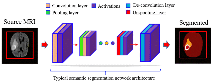
Description - Figure 2: Typical process of segmentation with Deep Learning with a Convolutional Neural Network. Image source: Going Deep in Medical Image Analysis: Concepts, Methods, Challenges and Future Directions.
Typical process of segmentation with Deep Learning with a Convolutional Neural Network (CNN) based model is learned that first compresses the source image with a stack of different convolution, activation and pooling layers.
Presently, CNNs are considered state-of-the-art networks for supervised DL image segmentation problems.Footnote 18 Their architecture is inspired by a hierarchical receptive field model of the visual cortex and generally includes the composition of three types of layers:
- Convolutional layers, where a kernel (filter) is convolved over inputs to extract a hierarchy of features,
- Nonlinear layers, which allow inputs to be mapped to feature spaces, and;
- Pooling layers, which reduce the spatial resolution by aggregating local information.
Each layer is made of processing units that are locally connected. These local connections are called receptive fields. The layers are typically composed to form a multi-resolution pyramid in which higher-level layers learn features from wider receptive fields. The model parameters are typically learned through a stochastic version of the backpropagation algorithm,Footnote 19 which is a gradient-based optimization routine that efficiently propagates the gradient of the residual through the network.
Evaluation Methods
Generally, supervised segmentation evaluation methods attempt to quantify the degree of overlap between an estimated and ground truth segmentation. Using the map notation of a segmentation in expression (2), we can equivalently understand the segmentation as a set with the image of its map, i.e.
The Dice score (D) is one of the most popular and conceptually easy to understand segmentation evaluation methods. For two segmentations and , the Dice score is calculated as follows
The Jaccard coefficient (J) is another segmentation evaluation method and is related to the Dice score through the following expression
is known to yield higher values for larger volumes. Another segmentation evaluation method is the average Hausdorff distance, which is especially recommended for segmentation tasks with complex boundaries and small thin segments and compared to the Dice score, the average Hausdorff distance has the advantage of accounting for localization when considering segmentation performance.Footnote 20 For two segmentations and , which are non-empty subsets of a metric space , the Average Hausdorff distance is calculated as follows
For more evaluation methods, the interested reader can consult Metrics for evaluating 3d medical image segmentationFootnote 22
Conclusion
To conclude, image segmentation is a crucial technique in image processing in general and medical imaging in particular. This process is an imperative part of an image processing pipeline which requires downstream image analyses, in which semantic substructures in an image are identified. Using machine learning we can automate this procedure while retaining the quality of an expert annotator and for the fraction of the cost.

If you have any questions about my article or would like to discuss this further, I invite you to Meet the Data Scientist, an event where authors meet the readers, present their topic and discuss their findings.
Thursday, November 17
2:00 to 3:00 p.m. EST
MS Teams – link will be provided to the registrants by email
Register for the Data Science Network's Meet the Data Scientist Presentation. We hope to see you there!
- Date modified: