Developments in Machine Learning Series: Series one

By: Nicholas Denis, Statistics Canada

This month's topics:

• A novel pre-training approach: Contrastive Language-Image Pre-training (CLIP)
• Neural network trained using batch normalization parameters
• Measuring Hard to Learn Data Instances and how this can be leveraged to train a neural network

Game Changer: There's a new pre-trained transfer learning approach in town!

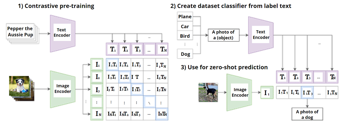
Figure 1: Contrastive Language-Image Pre-training (CLIP)

OpenAI introduces a novel pre-training approach producing state-of-the-art pre-trained models for computer vision

What's new?: CLIP uses both text and image inputs to train computer vision models, without any labels, which can perform a wide variety of tasks at (or near) state-of-the-art performance levels, across 30 different hold-out datasets. Some examples of tasks include object recognition, OCR, action recognition from videos, geo-localization and fine-grained object classification. OpenAi, the company that introduced the novel process, made the open-source models available publicly.

How it works: OpenAI built a web-scraped dataset containing 400 million instances of images paired with text descriptions. They introduce Contrastive Language-Image Pre-training (CLIP), which takes an image input and a text description of the image, and learns to embed the image and text representations onto the surface of a (hyper) sphere, as closely as possible. That's it!

Why does it work?: Imagine if you could identify text descriptions associated with 400 million different images? It would be fair to say that you've learned the semantics of objects in the images, and correctly identified a large number of categories and concepts. This is exactly what happens for CLIP. CLIP introduces a novel inference mechanism using textual prompts:

• since CLIP is trained without any labels, there is no classification layer present.
• for a given input image, CLIP produces an image embedding.
• for any given set of classes for given application, textual prompts enter the model in the form of "A photo of an <CLASS>", where CLASS is replaced with the classes of interest (ex. cat, dog).
• CLIP produces a text embedding for each prompt, and the closest to the image embedding is selected as the inferred class.

Results: After pre-training a model with a huge corpus of image-text data from the web, the authors use over 30 different benchmark computer vision datasets and study the performance of CLIP across a wide number of computer vision tasks. The authors test the model performance on zero-shot transfer learning (no further learning), as well as linear evaluation and fine-tuning.

• CLIP using zero-shot learning (where at inference time, a learning algorithm must perform classification on instances from classes not observed during training) outperforms a fully supervised linear classifier fitted to ResNet – 50 features on 16 out of 27 datasets, including ImageNet.
• Fitting a linear classifier on CLIP's features outperforms the Noisy Student EfficientNet-L2 (state-of-the-art transfer learning from ImageNet dataset) on 21 out of 27 datasets, as high as 23.6% accuracy improvement.
• CLIP zero-shot performance was incredibly robust to distributional shifts including adversarial attacks, stylized images, use of synthetic noise and use of synthetically rendered images.

What's the context?: OpenAI has helped to pioneer language model pre-training with the GPT family of language models which are commonly used. Clearly, their expertise in this area has helped them produce this novel approach. Since being published in early 2021, several dozen works have expanded, have been analyzed and used CLIP, making it the breakout work of 2021. The models and code are freely available online: openAI/CLIP GitHub. As stated on their website, OpenAI is an AI research and deployment company. Their mission is to ensure that artificial general intelligence benefits all of humanity. (AGI)—highly autonomous systems that outperform humans at most economically valuable work—benefits all of humanity. They attempt to directly build safe and beneficial AGI, make their work available to others aiming for the same outcome, and are governed by the OpenAI non-profit board.

So what?: CLIP has been used for image and video retrieval using text, segmentation and image captioning. While CLIP has other uses such as model fine-tuning, traditional transfer learning approaches (which involve freezing the CLIP model), or by using its features as inputs to a new, smaller neural network model; the valuable aspect of CLIP lies in its zero-shot transferability.

When CLIP was evaluated on ImageNet (1 million image dataset with 1,000 classes) it achieved 76.2% accuracy, with no class supervision. CLIP can act as an open-set classifier by using the text prompts. Rather than having a parametric model output, (a distribution over a fixed number of classes) , at inference time, CLIP is able to query the model with any number of classes using the novel prompt design. This makes it incredibly versatile and general.

Separate research using CLIP for segmentation shows that when given an image of zebras drinking along a riverbed, the text prompt reads "The zebra in front of the other zebras". This causes the CLIP model to properly segment the zebra asked of it. Truly game changing!

Our opinion: The literature speaks for itself. The number of research papers using CLIP shows just how novel and powerful it is. CLIP is useful for a wide range of computer vision tasks. We believe that deep learning approaches that use multiple data modalities (i.e. image/text/audio, etc.) will become increasingly common. However, as it's been noted with language model pre-training such as GPT-3 from OpenAI, it's likely that the size of these models will increase. As these models increase in parameter, only the largest tech companies will be able to afford the costs of training these models – making it unlikely for that they'll be open-source and also unlikely for public use.

BatchNorm is All You Need

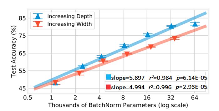
Figure 2: The relationship between BatchNorm parameter count and accuracy when scaling depth and width CIFAR-10 ResNets.

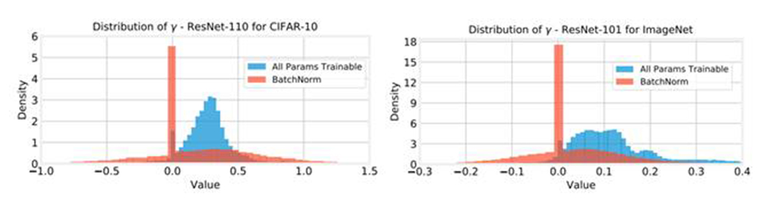
Figure 3: The distribution of y for ResNet-110 and ResNet-101 aggregated from five (CIFAR-10).

Researchers from MIT and Facebook Research achieve 83% accuracy on CIFAR10 training only batch norm parameters.

What's new?: Batch normalization is a ubiquitously implemented technique in deep learning. The authors study the expressive power of batch norm parameters by training neural networks, providing evidence that batch norm is extremely powerful in deep learning and capable of learning from random features.

How it works: Z-scoring is a common technique in data preprocessing, which aims to transform inputs to be approximately normal(0,1). However, in deep learning, as each batch of data passes through the network, the data is transformed at each layer and will no longer follow this distribution. Batch norm is similar to z-scoring, however, it doesn't aim to transform the data to be normal(0,1) but rather, normal$(\beta ,\gamma )$ where $\beta$ and $\gamma$ are learnable parameters. The authors train neural networks where all weight parameters are fixed and do not update, while the batch norm parameters are the sole parameters updated through learning.

Results:

• The authors first demonstrate that for different neural network architectures, using batch norm is consistently beneficial and improves model performance.
• When using a ResNet-110 on CIFAR10, with all 1.7 million parameters learnable, the model achieves 93.3% test accuracy, however when using only the 8300 batch norm parameters, the model is able to achieve 69.7% test accuracy. Moreover, a ResNet-866 with 65,000 parameters achieves 83% test accuracy.
• Using only batch norm parameters for learning, the authors found an almost perfect Pearson's correlation with batch norm parameters (layers of a network) and test accuracy.
• An analysis of the learned parameters showed that the model learns to effectively disable between a third and a quarter of all features, implicitly pruning the network.

What's the context?: Batch normalization has been the focus of many studies to determine why and how it works. Though, there aren't any deep learning practitioners who need any more evidence to use batch norm in their models. The fact that a model performs well using nothing but batch normalization is quite impressive and telling. Given that all other parameters are randomly initialized and fixed, this effectively means that the features produced from the input data are random, and batch norm parameters are able to iteratively transform the random features into discriminative features for downstream classification.

But…: Though the result is quite interesting and may result in further research, the authors are not suggesting practitioners train BatchNorm-only networks.

So what?: The implications of this work provide further support for the power and importance of using batch normalization in deep learning. An 866-layer ResNet with only 65,000 parameters is able to achieve very strong results, whereas a single layer network with that number of parameters would likely fail the same task. This result could very well open up novel architectural designs and research centered around deeper but narrower networks (less parameters per layer).

Our opinion: The research is interesting in its own right, and is important for the advancement of batch norm related research. Since each layers weights of the networks are randomly initialized, each layer acts as a random transformation on the data, producing random features. Given that batch norm learns solely to rescale and shift these random features, this work provides evidence that this approach may work well for transfer learning tasks using pre-trained models. As well, given that a large proportion of the learned parameters effectively pruned or disabled features, there may be some cross pollination with the Pruning Neural Networks community. As a take home for our readers, though, is the simple message: use batch normalization.

Measuring Hard to Learn Data Instances

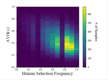
Figure 4: Human Selection Frequency vs. Angular Visual Hardness (HVS(x))

Researchers identify a measure of 'hardness' of a data instance to be correctly classified that negatively correlates with the frequency which human annotators select instances as examples of a given class.

What's new: Researchers from Universities of Toronto, Rice, Caltech, Georgia Institute of Tech, NVIDIA and the Vector Institute develop a measure of how difficult an example is with respect to a models ability to correctly classify it, and train the model using a curriculum based on this measure.

How it works: Angular Visual Hardness (AVH) computes the angle that an embedding makes with each of the class center and produces a score where, roughly speaking, larger values correspond to embeddings that have larger angles from the classes of their ground truth labels (and hence are further). Then, using AVH, the dataset can be ranked in terms of instance difficulty, and a subset can be used to train a model using instances of an appropriate difficulty level (curriculum learning).

Results:

• Researchers found that AVH strongly correlates (negatively) with Human Selection Frequency – the frequency at which human annotators would select an instance as an example of a given class. Hence, the easier the example, the more likely a human would select/recognize it as an example of a given class.
• Researchers use AVH for semi-supervised self-training in the domain adaptation setting. Briefly, this involves two completely different datasets generated from completely different distributions, however with the same classes. With labels on the 'source' dataset, and no training labels in the 'target' dataset, the goal is to generalize to unseen instances of the 'target' dataset. Models were firs trained on the 'source' dataset, and AVH was applied to the 'target' dataset. Instances below a threshold (easier instances) were selected to produce pseudo-labels by the previously trained models (see Pseudo-Labeling to deal with small datasets). These pseudo-labelled instances were added to the dataset and the model was re-trained. This approach outperformed previous state of the art domain adaption approaches across different datasets.

What's the context?: Curriculum learning is a widely studied field in machine learning. Hard and semi-hard sample mining techniques are crucial for many deep metric learning and self-supervised learning techniques.

So what?: From deep metric learning, to curriculum learning, measuring the difficulty of instances of a dataset have been increasingly important for a wide variety of machine learning techniques. Many real world datasets have noisy (read: incorrect) labels in the dataset, and likely (read: hopefully) the model never "correctly" classifies such instances. The field of identifying mislabelled instances use difficult examples to either adjust, relabel or remove from the dataset in order to improve model performance. Curriculum learning benefits from producing properly sequenced instances for the model to learn from, finding a "Goldilocks" level of difficulty. Instances that are too easy are a waste of compute power and don't produce valuable gradients for learning updates, while too difficult examples may be outliers, mislabelled, or simply unlikely to ever be correctly classified. In either case, both may be harmful to the model and a waste of compute power.

But…: Though AVH is novel in its exact formulation, using the angle between an embedding and its ground truth class center, or variants thereof, have existed before. However, this is the first work (to our knowledge) that shows a correlation between a hardness measure and how humans may judge an instance as being easy vs hard.

Our opinion: Though it is unlikely that AVH is adopted as the ultimate measure of instance hardness, the hopes of this article was to share that there is a large body of literature aiming to measure difficulty in training instances, and use this information to inform training in the form of loss functions, pseudo-labelling, anomaly detection and curriculum learning.