
MLflow Tracking: An efficient way of tracking modeling experiments
By: Mihir Gajjar, Statistics Canada
Contributors: Reginald Maltais, Allie Maclsaac, Claudia Mokbel and Jeremy Solomon, Statistics Canada
MLflow is an open source platform that manages the machine learning lifecycle, including experimentation, reproducibility, deployment and a central model registry. MLflow offers four components:
- MLflow Tracking: Record and query experiments—code, data, configuration parameters and results.
- MLflow Projects: Package data science code in a format to reproduce runs on any platform.
- MLflow Models: Deploy machine learning models in diverse serving environments.
- Model Registry: Store, annotate, discover and manage models in a central repository.
This article focuses on MLflow Tracking. The MLflow website has details on the remaining three components.
Benefits of MLFlow
MLflow Tracking provides a solution that can be scaled from your local machine to the entire enterprise. This allows data scientists to get started on their local machine while organizations can implement a solution that ensures long term maintainability and transparency in a central repository.
MLflow Tracking provides consistent and transparent tracking by:
- Tracking parameters and the corresponding results for the modeling experiments programmatically and comparing them using a user interface.
- Recovering the model having the best results along with its corresponding code for different metrics of interest across experiments for different projects.
- Looking back through time to find experiments conducted with certain parameter values.
- Enabling team members to experiment and share results collaboratively.
- Exposing the status of multiple projects in a singular interface for management along with all their details (parameters, output plots, metrics, etc.).
- Allowing tracking across runs and parameters through a single notebook, reducing time spent managing code and different notebook versions.
- Providing an interface for tracking both Python and R based experiments.
How do I flow between my experiments with MLflow?
This article focuses on using MLflow with Python. The MLflow QuickStart document has examples of its use with R for a local installation on a single machine. Organizations wishing to deploy MLflow across teams could also refer to the QuickStart document.
This article will explore an example of using MLflow with Python; however, to get the best understanding of how MLFlow works, it's useful to go through each step on your machine.
Install MLflow
MLflow can be installed as a standard Python package by typing the following command in a terminal window:
$ pip install mlflow
After the command has finished executing, you can type mlflow in your terminal and explore the available options. For example, you can try: mlflow –version to see the version installed
Launch MLflow server
It's recommended to have a centralized MLflow server for an individual, team or organization so that runs for different projects can be logged in one central place, segregated by experiments (different experiments for different projects). This will be covered in more detail later in this article. To quickly get started with the tool, you can skip the server launch and still log the runs. By doing this, the runs are stored in a directory called "MLruns" located in the same directory as the code. You can later open MLflow UI in the same path and visualize the logged runs.
The runs can be logged to an MLflow server running locally or remotely by setting the appropriate tracking URI (uniform resource identifier). Setting the appropriate logging location is explained later.
If, however, you prefer to start the server right away, you can do so by issuing the following command:
$ mlflow server
The terminal will display information similar to what is below, which shows the server is listening at localhost port 5000This address is useful for accessing the MLflow user interface (UI). Feel free to explore the subtle difference between MLflow UI and MLflow server in the MLflow Tracking documentation.
[2021-07-09 16:17:11 –0400] [58373] [INFO] Starting gunicorn 20.1.0
[2021-07-09 16:17:11 –0400] [58373] [INFO] Listening at: http://127.0.0.1:5000 (58373)
[2021-07-09 16:17:11 –0400] [58373] [INFO] Using worker: sync
[2021-07-09 16:17:11 –0400] [58374] [INFO] Booting worker with pid: 58374
[2021-07-09 16:17:11 –0400] [58375] [INFO] Booting worker with pid: 58375
[2021-07-09 16:17:11 –0400] [58376] [INFO] Booting worker with pid: 58376
[2021-07-09 16:17:11 –0400] [58377] [INFO] Booting worker with pid: 58377
Logging data to MLflow
There are two main concepts in MLflow tracking: experiments and runs. The data logged during an experiment is recorded as a run in MLflow. The runs can be organized into experiments, which groups together runs for a specific task. One can visualize, search, compare, and download run artifacts and metadata for the runs logged in an MLflow experiment.
Data in an experiment can be logged as a run in MLflow using MLflow Python, R, Java packages, or through the REST API (application programming interface).
This article will demonstrate modeling for one of the "Getting started with NLP (natural language processing)" competitions on Kaggle called "Natural Language Processing with Disaster Tweets." A Jupyter notebook and the MLflow Python API will be used for logging data to MLflow. The focus will be on demonstrating how to log data to MLflow during modeling, rather than getting the best modeling results.
First, let's start with the usual modeling process, which includes imports, reading the data, text pre-processing, tf-idf (term frequency-inverse document frequency) features and support vector machine (SVM) model. At the end, there will be a section called "MLflow logging."
Note: The NLP pipeline is kept as simple as possible so that the focus is on MLflow logging. Some of the usual steps, like exploratory data analysis, are not relevant for this purpose and will be left out. The preferred way of logging data to MLflow is by leaving a chunk of code at the end to log. You can also configure MLflow at the beginning of the code and log data throughout the code, when the data or variable is available to log. An advantage to logging all the data together at the end using a single cell is that the entire pipeline would finish successfully, and the run will log the data (given the code for MLflow logging has no bugs). If the data are logged throughout the code and the code execution stops for any reason, the data logging will be incomplete. However, if there's a scenario where a code has more than one code chunk, which takes a significant amount of time to execute, then logging throughout the code, in multiple locations, may actually be beneficial.
Importing the libraries
Start by importing all the required libraries for the example:
# To create unique run name.
import time
# To load data in pandas dataframe.
import pandas as pd

# NLP libraries

# To perform lemmatization
from nltk import WordNetLemmatizer
# To split text into words
from nltk. tokenize import word_tokenize
# To remove the stopwords
from nltk.corpus import stopwords

# Scikit-learn libraries

# To use the SVC model
from sklearn.svm import SVC
# To evaluate model performance
from sklearn.model_selection import cross_validate, StratifiedkFold
# To perform Tf-idf vectorization
from sklearn.feature_extraction.text import TfidfVectorizer
# To get the performance metrics
from sklearn.metrics import f1_score, make_scorer
# For logging and tracking experiments
import mlflow
Create a unique run name
MLflow tracks multiple runs of an experiment through a run name parameter. The run name can be set to any value, but should be unique so you can identify it amongst different runs later. Below, a timestamp is used to guarantee a unique name.
run_name = str(int(time.time()))
print('Run name: ', run_name)
Gives:
Run name: 1625604741Reading the data
Load the training and test data from the CSV files provided by the example.
# Kaggle competition data download link: https://www.kaggle.com/c/nlp-getting-started/data
train_data = pd.read_csv("./data/train.csv")
test_data = pd.read_csv("./data/test.csv")
By executing the following piece of code in a cell:
train_data
A sample of the training data that was just loaded can be seen in Figure 1.
Figure 1: A preview of the training data that was loaded.
![]()
Figure 1: A preview of the training data that was loaded.
The top and bottom five entries of the CSV file. It contains the columns: id, keyword, location, text and target. The text column contains the tweet itself and the target column, the class.
| id | keyboard | location | text | target | |
|---|---|---|---|---|---|
| 0 | 1 | NaN | Nan | Our Deeds are the Reason of this #earthquake M… | 1 |
| 1 | 4 | NaN | Nan | Forest fire near La Ronge Sask. Canada | 1 |
| 2 | 5 | NaN | Nan | All residents asked to 'shelter in place' are… | 1 |
| 3 | 6 | NaN | Nan | 13,000 people receive #wildfires evacuation or… | 1 |
| 4 | 7 | NaN | Nan | Just got sent this photo from Ruby #Alaska as… | 1 |
| ... | ... | ... | ... | ... | ... |
| 7608 | 10869 | NaN | Nan | Two giant cranes holding a bridge collapse int… | 1 |
| 7609 | 10870 | NaN | Nan | @aria_ahrary @TheTawniest The out of control w… | 1 |
| 7610 | 10871 | NaN | Nan | M1.94 [01:04 UTC] ?5km S of Volcano Hawaii. Htt… | 1 |
| 7611 | 10872 | NaN | Nan | Police investigating after an e-bike collided… | 1 |
| 7612 | 10873 | NaN | Nan | The Latest: More Homes Razed by Northern Calif… | 1 |
7613 rows x 5 columns
The training data are about 70% of the total data.
print('The length of the training data is %d' % len(train_data))
print('The length of the test data is %d' % len(test_data))
Output:
The length of the training data is 7613
The length of the test data is 3263
Text pre-processing
Depending on the task at hand, different types of preprocessing steps might be required to make the machine learning model learn better features. Preprocessing can normalize the input, remove some of the common words if required so that the model does not learn them as features, make logical and meaningful changes that can lead to the model performing and generalizing better. The following demonstrates how performing some pre-processing steps can help the model grab the right features when learning:
def clean_text(text):
    # split into words
    tokens = word_tokenize(text)
    # remove all tokens that are not alphanumeric. Can also use .isalpha() here if do not want to keep numbers.
    words = [word for word in tokens if word.isalnum()]
    # remove stopwords
    stop_words = stopwords.words('english')
    words = [word for word in words if word not in stop_words]
    # performing lemmatization
    wordnet_lemmatizer = WordNetLemmatizer()
    words = [wordnet_lemmatizer.lemmatize(word) for word in words]
    # Converting list of words to string
    words = ' '.join(words)
    return words
train_data['cleaned_text'] = train_data['text'].apply(clean_text)
Comparing the original text to the cleaned text, non-words have been removed:
train_data['text'].iloc[100]
'.@NorwayMFA #Bahrain police had previously died in a road accident they were not killed by explosion https://t.co/gFJfgTodad'
train_data['cleaned_text'].iloc[100]rain_data['text'].iloc[100]
'NorwayMFA Bahrain police previously died road accident killed explosion http'
Reading the text above, one can say that, yes, it does contain information about a disaster and hence should be classified as one. To confirm this with the data, print out the label present in the CSV file for this tweet:
train_data['target'].iloc[100]
Output:
1
Tf-idf features
Next, we are converting a collection of raw documents to a matrix of TF-IDF features to feed into the model. For more information about tf-idf, please refer to tf–idf - Wikipedia and scikit-learn sklearn.feature_extraction.text documentation.
ngram_range=(1,1)
max_features=100
norm='l2'
tfidf_vectorizer = TfidfVectorizer(ngram_range=ngram_range, max_features=max_features, norm=norm)
train_data_tfidf = tfidf_vectorizer.fit_transform(train_data['cleaned_text'])
train_data_tfidf
Output:
<7613x100 sparse matrix of type '<class 'numpy.float64'>'
with 15838 stored elements in Compressed Sparse Row format>
tfidf_vectorizer.get_feature_names()[:10]
Output:
['accident',
'amp',
'and',
'as',
'attack',
'back',
'best',
'body',
'bomb',
'building']
SVC model
The next step to perform the modeling is to fit a model and evaluate the performance.
Stratified K-Folds cross-validator is used to evaluate the model. See scikit learn sklearn.model_selection for more information.
strat_k_fold = StratifiedKFold(n_splits=5, shuffle=True, random_state=42)
Making a scorer function using the f1-score metric to pass it as a parameter in the SVC model.
scoring_function_f1 = make_scorer(f1_score, pos_label=1, average='binary')
Now comes an important step of fitting the model to the data. This example uses the SVC classifier. See scikit learn sklearn.svm.svc for more information.
C = 1.0
kernel='poly'
max_iter=-1
random_state=42
svc = SVC(C=C, kernel=kernel, max_iter=max_iter, random_state=random_state)
cv_results = cross_validate(estimator=svc, X=train_data_tfidf, y=train_data['target'], scoring=scoring_function_f1, cv=strat_k_fold, n_jobs=-1, return_train_score=True)
cv_results
Output:
{'fit_time': array([0.99043322, 0.99829006, 0.94024873, 0.97373009, 0.96771407]),
'score_time': array([0.13656974, 0.1343472 , 0.13345313, 0.13198996, 0.13271189]),
'test_score': array([0.60486891, 0.65035517, 0.5557656 , 0.5426945 , 0.63071895]),
'train_score': array([0.71281362, 0.76168757, 0.71334394, 0.7291713 , 0.75554698])}
def mean_sd_cv_results(cv_results, metric='F1'):
    print(f"{metric} Train CV results: {cv_results['train_score'].mean().round(3)} +- {cv_results['train_score'].std().round(3)}")
    print(f"{metric} Val CV results: {cv_results['test_score'].mean().round(3)} +- {cv_results['test_score'].std().round(3)}")

mean_sd_cv_results(cv_results)
F1 Train CV results: 0.735 +- 0.021
F1 Val CV results: 0.597 +- 0.042
Note: The code below is executed as a shell command by adding the exclamation mark: '!' in the beginning of the code in a Jupyter cell.
! Jupyter nbconvert --to html mlflow-example-real-or-not-disaster-tweets-modeling-SVC.ipynb
[NbConvertApp] Converting notebook mlflow-example-real-or-not-disaster-tweets-modeling-SVC.ipynb to html
[NbConvertApp] Writing 610630 bytes to mlflow-example-real-or-not-disaster-tweets-modeling-SVC.html
Logging to MLflow
First, set the server URI. As the server is running locally, set the tracking URI to localhost port 5000. The tracking URI can be set to a remote server as well (see Where Runs are Recorded).
server_uri = 'http://127.0.0.1:5000'
mlflow.set_tracking_uri(server_uri)
To organize the runs, an experiment was created and set where the runs will be logged. The "set_experiment" method will create a new run with the given string name and set it as the current experiment where the runs will be logged.
mlflow.set_experiment('nlp_with_disaster_tweets')Finally, start a run and log data to MLflow.
# MLflow logging.
with mlflow.start_run(run_name=run_name) as run:

    # Logging tags
    # run_name.
    mlflow.set_tag(key='Run name', value=run_name)
    # Goal.
    mlflow.set_tag(key='Goal', value='Check model performance and decide whether we require further pre-processing/hyper-parameter tuning.')
    # Modeling exp.
    mlflow.set_tag(key='Modeling technique', value='SVC')

    # Logging parameters
    mlflow.log_param(key='ngram_range', value=ngram_range)
    mlflow.log_param(key='max_features', value=max_features)
    mlflow.log_param(key='norm', value=norm)
    mlflow.log_param(key='C', value=C)
    mlflow.log_param(key='kernel', value=kernel)
    mlflow.log_param(key='max_iter', value=max_iter)
    mlflow.log_param(key='random_state', value=random_state)

    # Logging the SVC model.
    mlflow.sklearn.log_model(sk_model=svc, artifact_path='svc_model')

    # Logging metrics.
    # mean F1-score - train.
    mlflow.log_metric(key='mean F1-score - train', value=cv_results['train_score'].mean().round(3))
    # mean F1-score - val.
    mlflow.log_metric(key='mean F1-score - val', value=cv_results['test_score'].mean().round(3))
    # std F1-score - train.
    mlflow.log_metric(key='std F1-score - train', value=cv_results['train_score'].std().round(3))
    # std F1-score - val.
    mlflow.log_metric(key='std F1-score - val', value=cv_results['test_score'].std().round(3))

    # Logging the notebook.
    # Nb.
    mlflow.log_artifact(local_path='real-or-not-disaster-tweets-modeling-SVC.ipynb', artifact_path='Notebook')
    # Nb in HTML.
    mlflow.log_artifact(local_path='real-or-not-disaster-tweets-modeling-SVC.html', artifact_path='Notebook')
In the code above, you begin a run with a run_name and then log the following:
- Tags: A key-value pair. Both the key and the value are strings. For instance, this can be used to log the goal of the run where the key would be 'Goal:' and the value can be 'To try out the performance of Random Forest Classifier with default parameters.'
- Parameters: Also, a key-value pair and can be used to log the model parameters.
- Model: Can be used to log the model. Here you are logging a scikit-learn model as an MLflow artifact, but we can also log a model for other supported machine learning libraries using the corresponding MLflow module.
- Metrics: A key-value pair. The key data type is "string" and it can have the metric name. The value parameter has a data type "float". The third optional parameter is "step" which is an integer that represents any measurement of training progress – number of training iterations, number of epochs, etc.
- Artifacts: A local file or directory can be logged as an artifact for the current run. In this example, we're logging using the notebook so that they're accessible for future runs. By doing this, you can save a plot like "loss curve" or "accuracy curve" in the code and log them as an artifact in MLflow.
There you have it—you successfully logged data for a run in MLflow! The next step is to visualize the logged data.
MLflow UI
If you scroll back to Figure 1, you'll remember that you launched the server and it was listening at localhost port 5000. Open this address in your preferred browser to access the MLflow UI. Once the MLflow UI is visible, you can use the interface to look at the experiment data that was logged. The experiments created appear in the sidebar of the UI, and the logged tags, parameters, model and metrics are shown in the columns.
Figure 2: MLflow UI
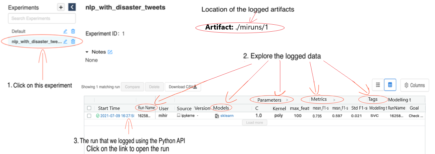
Figure 2: MLflow UI
Figure 2 shows the MLflow UI. The experiment which was set above i.e. nlp_with_disaster_tweets is opened and the run that you logged earlier along with the details such as run name, parameters and metrics. It also shows the location where the artifacts are stored. You can click on the logged run to explore it in further detail.
Text in image: MLflow Expriements Models
Nlp_with_disaster_tweets (1. Click on this experiment)
Experiment ID: 1, Artifact Location: ./miruns/1 (Location of the logged artifacts)
Notes: None
2. Explore the logged data
| Parameters | Metrics | Tags | ||||||||||
|---|---|---|---|---|---|---|---|---|---|---|---|---|
| Start Time | Run Name | User | Source | Version | Model | C | Kernel | max_feature | Mean F1-s | Mean F1-s | Std F1-s | Modeling t |
| 2021-07-09 16:27:58 | 16258… | Mihir | ipykerne | - | sklearn | 1.0 | poly | 100 | 0.735 | 0.597 | 0.021 | SVC |
3. The run that we logged using the Python API. Click on the link to open the run
To explore a specific run in greater detail, click on the relevant run in the Start Time column. This will allow you to explore a logged run in detail. The run name is shown and you can add any notes for the run such as logged parameters, metrics, tags and artifacts. The data logged using the Python API for this run are shown here.
The files logged as artifacts can be downloaded, which can be useful if you want to retrieve the code later. Since the code that generates results for every run is saved, you don't need to create multiple copies of the same code and can experiment using a single skeleton notebook by changing the code between runs.
The logged trained model can be loaded in a future experiment using the Python API from the logged run.
Figure 3: Exploring the logged artifacts in a run
![]()
Figure 3: Exploring the logged artifacts in a run
Figure 3 explores the logged artifacts. The logged files (notebook and the model) are shown. The description of the model also provides code to load the logged model in Python.
Text in image:
Tags
| Name | Value | Actions |
|---|---|---|
| Goal | Check model performance and decide whether we require further pre-processing hyper-parameter tuning. | Edit – delete icons |
| Modeling technique | SVC | Edit – delete icons |
| Run name | 16525862471 | Edit – delete icons |
Add Tag
Name – Value – Add
Artifacts
Notebook
- Real-or-not-disaster-tweets-modeling-SVC.html
- Real-or-not-disaster-tweets-modeling-SVC.ipynb
svc_model
- MLmodel
- conda.yaml
- model.pld
Full Path: ./miruns/1/fcdc8362b2fe74329a4128fa522d80cb/artifacts/svc_model
Size: 0B
MLflow Model
The code snippets below demonstrate how to make predictions using the logged model
Model schema
Input and output schema for your model. Learn more
Name – Type
No Schema.
To demonstrate the run comparison functionality, more modeling experiments were performed and logged to MLflow by changing a few parameters in the same jupyter notebook. Feel free to change some parameters and log more runs to MLflow.
Figure 4 shows the different logged runs. You can filter, keep the columns you want, and compare the parameters or metrics between different runs. To perform a detailed comparison, you can select the runs you want to compare and click on the "Compare" button highlighted in the figure below.
Figure 4: Customizing and comparing different runs using MLflow UI
![]()
Figure 4: Customizing and comparing different runs using MLflow UI
In MLflow UI, one can customize the columns being shown, filter and search for different runs based on the logged data and can easily compare the different logged runs based on the visible columns. You can also compare different logged runs in greater detail by selecting them and clicking on the "Compare" button.
Text in image:
1. Can filter and keep the columns of interest
Columns: Start Time, User, Run Name, Source, Version, Models, Parameters, Metrics, Tags
2. Can compare different runs
3. Different runs logged. Select the runs you want to compare
Showing 5 matching runs. Compare, Delete, Download, CSV
4. Click Compare
| Parameters | Metrics | Tags | ||||||||||||
|---|---|---|---|---|---|---|---|---|---|---|---|---|---|---|
| Start Time | Run Name | User | Source | Version | Model | C | Kernel | max_fe | Mean F1-s | Mean F1-s | Std F1-s | Modeling | Run name | Goal |
| 2021-07-12 14:48:54 | 1626115725 | Mihir | ipykerne | - | sklearn | 1.0 | Poly | 500 | 0.93 | 0.694 | 0.001 | SVC | 16261157 | Check mo… |
| 2021-07-12 14:48:16 | 1626115688 | Mihir | ipykerne | - | sklearn | 1.0 | Poly | 500 | 0.931 | 0.693 | 0.001 | SVC | 16261156 | Check mo… |
| 2021-07-12 14:48:50 | 1626115602 | Mihir | ipykerne | - | sklearn | 1.0 | Poly | 500 | 0.933 | 0.694 | 0.002 | SVC | 16261156 | Check mo… |
| 2021-07-12 14:48:01 | 1626115552 | Mihir | ipykerne | - | sklearn | 1.0 | Poly | 500 | 0.876 | 0.649 | 0.002 | SVC | 16261155 | Check mo… |
| 2021-07-09 16:27:58 | 1625002471 | Mihir | ipykerne | - | sklearn | 1.0 | Poly | 500 | 0.735 | 0.597 | 0.021 | SVC | 16258624 | Check mo… |
After clicking the "Compare" button, a table-like comparison between different runs will be generated, (as shown in Figure 5) allowing you to easily compare logged data across different runs. The parameters that differ across the runs are highlighted in yellow. This gives the user an idea of how model performance has changed over time based on the change in parameters.
Figure 5: Comparing logged runs in MLflow UI in detail
![]()
Figure 5: Comparing logged runs in MLflow UI in detail
Figure 5 compares different logged runs in MLflow in detail. The tags, parameters and metrics are in different rows and the runs are in different columns. This allows a user to compare details of interest for different runs in a single window. The parameters which are different in different runs are highlighted in yellow. For example, in the experiments the parameters max_features and ngram_range were changed for different runs and hence they are highlighted in yellow in the image above.
Text in image:
Nlp_with_disaster_tweets > Comparing 5 Runs
| Run ID: | 7a1448a5f88147c093 c357d787dbe3 |
264533b107b04be3 bd4981560bad0397 |
7670578718b3477abb 798d7e404fed6c |
D2372d5873f2435c 94dc7e633a611889 |
Fdc8362b2f37432f9 a4128fa522d80cb |
|---|---|---|---|---|---|
| Run Name | 1626115725 | 1626115688 | 1626115602 | 1626115552 | 16265862471 |
| Start Time | 2021-07-12 14:48:54 | 2021-07-12 14:48:16 | 2021-07-12 14:48:50 | 2021-07-12 14:46:01 | 2021-07-09 16:27:58 |
| Parameters | |||||
| C | 1.0 | 1.0 | 1.0 | 1.0 | 1.0 |
| Kernel | Poly | Poly | Poly | Poly | Poly |
| Max_features | 500 | 500 | 500 | 500 | 500 |
| Max_iter | -1 | -1 | -1 | -1 | -1 |
| Ngram_range | (1.3) | (1.2) | (1.1) | (1.1) | (1.1) |
| Norm | 12 | 12 | 12 | 12 | 12 |
| random_state | 42 | 42 | 42 | 42 | 42 |
| Metrics | |||||
| Mean f1-score-train | 0.93 | 0.931 | 0.933 | 0.876 | 0.735 |
| Mean f1-score-val | 0.694 | 0.693 | 0.694 | 0.649 | 0.597 |
| std f1-score-train | 0.001 | 0.001 | 0.002 | 0.002 | 0.021 |
| std f1-score-val | 0.008 | 0.009 | 0.01 | 0.013 | 0.042 |
Changes in the parameters and metrics across different runs can also be laid-out in a Scatter Plot. The values of the x-axis and y-axis can be set to any parameter or metric allowing the user to analyze the changes. In Figure 6, the reader can analyze the change in validation, in this case the mean F1-score, over different values for the parameter 'max_features'. If you hover over a data point, you can see details about that run.
Figure 6: Configuring the scatter plot to visualize the effects of different parameter configurations in the logged runs
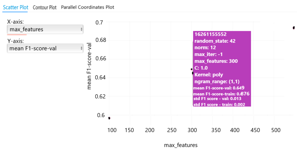
Figure 6: Configuring the scatter plot to visualize the effects of different parameter configurations in the logged runs
A demonstration of MLflow's capability of plotting a graph using details from different runs. You can select a particular parameter on X-axis and a metric you want to monitor on the Y-axis; this will create a scatter plot with the details on the corresponding axis on the go and you will be able to visualize the effects of the parameter on the metric to get an idea about how the parameter is affecting the metric.
Text in image:
Scatter Plot
X-Axis: max_features
Y-Axis: mean F1-score-val
| Run Name | 1626115552 |
|---|---|
| Start Time | 2021-07-12 14:46:01 |
| C | 1.0 |
| Kernel | Poly |
| Max_features | 500 |
| Max_iter | -1 |
| Ngram_range | (1.1) |
| Norm | 12 |
| random_state | 42 |
| Mean f1-score-train | 0.876 |
| Mean f1-score-val | 0.649 |
| std f1-score-train | 0.002 |
| std f1-score-val | 0.013 |
The Parallel Coordinates Plot is also useful, as it shows the viewer the effect of the selected parameters on the desired metrics at a glance.
Figure 7: Configuring the parallel coordinates plot to visualize the effects of different parameters on the metrics of interest
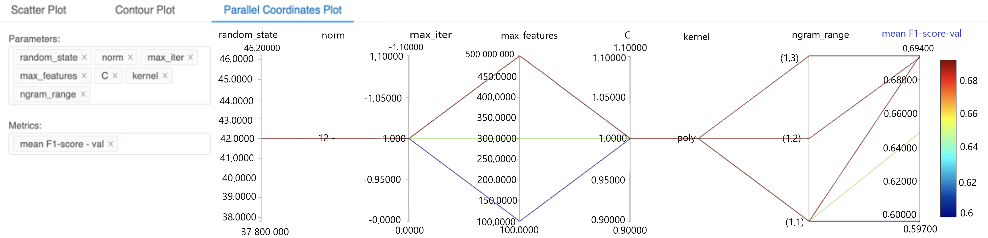
Figure 7: Configuring the parallel coordinates plot to visualize the effects of different parameters on the metrics of interest
In this image a parallel coordinates plot is configured. You can select different parameters and metrics using the provided input windows, based on which the parallel coordinates plot is updated. This plot can provide an idea about the results you get using different configurations in the experiments. It can help in comparing different configurations and selecting the parameters that perform better.
Text in image:
Scatter Plot – Contour Plot – Parallel Coordinates Plot
Paramters: random_state, norm, max_iter, max_features, C, kernel, ngram_range
Metrics: mean F1-score-val
| random_state | norm | Max_iter | Max_features | C | Kernel | ngram_range | Mean F1-score-val | |
|---|---|---|---|---|---|---|---|---|
| 46.20000 | -1.10000 | 500.00000 | 1.10000 | 0.69400 | ||||
| 46.0000 | -1.10000 | 500.00000 | 1.10000 | (1.3) | 0.68000 | 0.68 | ||
| 45.0000 | 450.00000 | |||||||
| 44.0000 | -1.05000 | 400.00000 | 1.05000 | 0.66000 | 0.66 | |||
| 43.0000 | 350.00000 | |||||||
| 42.0000 | -1.0000 | 300.00000 | 1.00000 | poly | (1.2) | 0.64000 | 0.64 | |
| 41.0000 | 250.00000 | |||||||
| 40.0000 | -0.95000 | 200.00000 | 0.95000 | 0.62000 | 0.62 | |||
| 39.0000 | 150.00000 | |||||||
| 38.0000 | -0.9000 | 100.00000 | 0.90000 | (1.1) | 0.60000 | 0.6 | ||
| 37.80000 | -0.90000 | 100.0000 | 0.9000 | 0.59700 |
Other interesting stuff in MLflow tracking:
There are other important points to note with MLflow tracking:
- The runs can be exported to a CSV file directly using the MLflow UI.
- All functions in the tracking UI can be accessed programmatically—you can query and compare runs with code, load artifacts from logged runs or run automated parameter search algorithms by querying the metrics from logged runs to decide the new parameters. You can also log new data to an already logged run in an experiment after loading it programmatically (visit Querying Runs Programmatically for more information).
- By using the MLflow UI, users can search for runs having specific data values using the search bar. An example of this would be to use
metrics.rmse < 1andparams.model='tree'. This is very helpful when you need to dig up a run with specific parameters executed in the past. - The Jupyter notebook used as an example in this blog post can be found on GitHub.
Feel free to contact us at statcan.dsnfps-rsdfpf.statcan@statcan.gc.ca and let me know about other interesting features or use case you like to use that you feel could have been mentioned. We will also have an opportunity for you to Meet the Data Scientist to discuss MLFlow in greater detail. See below for more details.

If you have any questions about this article or would like to discuss this further, we invite you to our new Meet the Data Scientist presentation series where the author will be presenting this topic to DSN readers and members.
Tuesday, October 18
2:00 to 3:00 p.m. EDT
MS Teams – link will be provided to the registrants by email
Register for the Data Science Network's Meet the Data Scientist Presentation. We hope to see you there!
- Date modified: