
By Pierre Zwiller-Panicz, Margarita Novikova, Kirsten Gaudreau, Matthew Paslawski, Housing, Infrastructure and Communities Canada.
Summary
This study develops and implements a machine learning model to forecast expenditures in HICC Grants and Contributions programs, focusing on reimbursement-based claims. A comparative analysis of algorithms identified Random Forest as the most effective, achieving an R-squared of 39%. Integrated into a Power BI dashboard, the model enables real-time expenditure analysis, trend visualization, and actual vs. forecast comparisons. Its implementation reduced forecasting time from three months to one, improving financial planning and stakeholder engagement.
The model has had a significant business impact, streamlining discussions between financial managers (FMAs) and program stakeholders while providing real-time insights for better decision-making. Although its applicability is limited to programs with established projects and it performs less accurately for allocation-based programs, it has proven highly effective for reimbursement-based claims with 30 or more active projects.
With its demonstrated success, the model represents a valuable step forward in financial forecasting. Its implementation has set the stage for further advancements, paving the way for broader adoption and continued improvements in predictive accuracy and program applicability.
1. Introduction
Housing, Infrastructure, and Communities Canada plays a crucial role in funding and supporting infrastructure projects that contribute to sustainable, inclusive, and climate-resilient communities. The department’s G&C programs require detailed, multi-year financial forecasts to ensure efficient allocation of government funding. However, the unpredictable nature of infrastructure projects often leads to overstated cashflow estimates, resulting in unspent funds and budget inefficiencies. As HICC's G&C programming continues to expand, the need for a scalable, data-driven forecasting solution has become increasingly clear.
To address these challenges, HICC implemented a ML forecasting model in May 2024. This innovative tool leverages advanced analytics to improve expenditure forecasting, enhance financial planning accuracy, and optimize budget allocation. By integrating this model into HICC’s existing suite of forecasting tools, the department aims to reduce inefficiencies, support data-driven decision-making, and strengthen its ability to fund critical infrastructure initiatives.
This article explores the development and implementation of the ML G&C forecasting model. It begins with an overview of the project’s background and objectives, followed by the model’s technical development and integration into HICC’s financial forecasting processes. The results and their impact on financial planning are then analyzed. The article concludes with recommendations for future enhancements and potential applications of the model.
2. ML Forecasting Model Background
2.1. Background and Evolution of Initiatives
In fiscal year 2016-2017 and 2017-2018, HICC lapsed approximately 64% of its anticipated Grants and Contributions authorities which led to a demand by central agencies for predictability in forecasting the fiscal profile of infrastructure programming. In response, HICC took several steps toward addressing these challenges:
- 2019–2020: HICC established a departmental Tiger Team to examine all aspects of the management of contribution funding to better align appropriations with actual expenditures.
- 2020–2022: HICC established a Grants and Contributions Centre of Expertise with a finance-focused skill set to address these issues.
2.2. Challenges in Current G&C Forecasting
Since its inception, the GCCOE has developed a suite of forecasting methods and processes that has helped reduce the departmental lapse in Grants Contribution funding. However, these methods and processes have created extensive workload on Financial Management Advisors (FMAs) to generate accurate forecasts which lacked standardization between different programs.
2.3. Purpose and Objective of the Model
To address these gaps, the GCCOE partners with the OCDO to explore a data-driven approach which could complement and build upon HICC’s existing suite of forecasting methods by providing a more accurate basis for FMA forecasts while simultaneously reducing workload.
The ML model's key objective is to improve forecasting of G&Cs at HICC by developing an automated forecasting tool informed by historical G&C data that is adaptable to current and new programming, thereby improving efficiency of HICC’s G&C multi-year forecasting process.
3. ML Forecasting Model Development & Implementation
This section will explore the development of the ML forecasting model, from its data sources to the final interactive tool. It will detail how the model was designed, integrated, and deployed to provide FMAs with real-time insights.
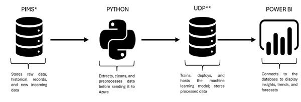
Description - Figure 1 : Data Pipeline
Description: The image illustrates a data pipeline: Program Information Management System (PIMS) stores raw and historical data, which is extracted, cleaned, and preprocessed in Python before moving to Azure. The Unified Data Platform (UDP) manages model training, deployment, and processed data storage. Finally, Power BI connects to the database to visualize insights.
3.1. Data Sources
The first step in developing the ML Forecasting Model involved sourcing data from HICC’s Program Information Management System (PIMS), as illustrated in Figure 1 – Data Pipeline. PIMS provided detailed information on program funding and expenditures across three layers: Programs, Contribution Agreements, and Projects. Key variables included:
| Variable | Definition | Sample Data |
|---|---|---|
| Project ID | A unique identifier for each project | 13176 |
| Contribution Agreement ID | A unique identifier linking the project to a specific funding agreement. | 2 |
| Fiscal Year | The fiscal year associated with the project’s expenditures and cashflows. | 2007-2008 |
| Project Cashflow | The projected or actual cash inflow and outflow for the project. | 500 000 |
| Project Expenditure | The amount spent on the project within a given period. | 500 000 |
| Total Amount per Contribution Agreement | The full allocated budget under a specific agreement. | 2 000 000 |
| Total Amount per Program Contribution | The overall funding contribution assigned to the program, encompassing multiple agreements. | 2 000 000 |
| Project Status | Indicates the current state of the project (e.g., active, completed, pending). | Closed |
3.2. Data Preprocessing
3.2.1. Cleansing and Transformation
The data cleaning process began by identifying and removing blank entries that were irrelevant to the financial forecasting model. The final dataset included only projects with statuses—"closed," "completed," and "in implementation"—ensuring a comprehensive evaluation across all stages of the project lifecycle, which enhanced the model's robustness and adaptability.
Next, data manipulation was performed to generate key variables such as average expenditure, prior expenditures, remaining amounts, and contribution agreement values. Finally, a disaggregation process standardized the data to a consistent level of granularity. Initially structured at multiple levels—project, contribution agreement, and program—the dataset was ultimately consolidated at the project level to align with the forecasting model’s analytical framework.
To enhance the model's ability to capture financial constraints and monitor spending limits, several engineered features were derived from existing variables. These features include the total project amount, cumulative project amount, cumulative previous expenditures, recent expenditures, project lifecycle, average preceding expenditures, remaining funds, and remaining funds at the start of each fiscal year. By integrating these variables, the dataset was enriched with additional financial insights, ensuring a more accurate representation of project spending dynamics.
| New Variables | Definition |
|---|---|
| Total Project Amount | The total budget allocated for a project over its entire duration. This is the sum of all planned expenditures for the project. |
| Cumulative Project Amount | The total amount spent on the project from its start up to the current fiscal year. This helps track how much of the budget has been utilized. |
| Cumulative Previous Expenditures | The sum of expenditures from all previous years before the current fiscal year. This excludes spending in the current year but provides historical financial context. |
| Recent Expenditures | The expenditures from the most recent fiscal year, reflecting the latest spending trends. |
| Project Lifecycle | The total number of years the project is expected to run, from its start year to its planned completion. |
| Average Preceding Expenditures | The average amount spent per year in past years. This is calculated as Cumulative Previous Expenditures / (Current Year - Start Year). |
| Remaining Funds | The total project budget minus cumulative expenditures. This represents the funds still available for future spending. |
| Remaining Funds at the Start of Each Fiscal Year | The amount of money left unspent at the beginning of a new fiscal year, before any new expenditures are incurred. |
| Amount | A derived variable used to improve forecast accuracy. Since future expenditures are initially 0, the model tends to predict unrealistically low values. Instead, the Amount variable replaces missing future expenditures with Cashflow (expected future disbursements), while keeping past expenditures unchanged. |
3.2.2. Segmentation
With the cleaned and transformed dataset in place, the next step involved analyzing the distribution of project expenditure to better inform the modeling approach. As illustrated in Figure 2 – Project Amount Distribution, the dataset exhibited significant heterogeneity, with 95% of projects accounting for only 5% of the department’s total dollar contribution, while the remaining 5% represented 95% of the expenditures.
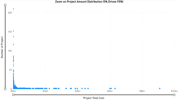
Figure 2: Project Amount Distribution
The scatter plot shows how project total costs relate to the number of projects. Most data points are clustered toward the lower end of the cost scale, meaning many projects have relatively low total costs. However, a few points are spread far to the right, indicating some projects have very high costs. This creates a right-skewed pattern, where the majority of projects are on the lower end, but a small number of high-cost projects extend the distribution.
Given the significant disparities in project expenditures our finance colleagues initially recommended a segmentation approach. Their manual classification was based on project amounts to account for this imbalance. To refine this approach, we explored an advanced segmentation methodology. Instead of segmenting by project amount, our analysis suggested that project duration provided a better differentiation because, when comparing results, project duration offered better homogeneity within clusters, leading to more consistent groupings and improved predictive performance. During the development phase, shifting the segmentation criterion from total project cost to project duration reduced the MAE for the Random Forest model by at least 300,000. This initial categorization of projects into high materiality (>5 years) and low materiality (<5 years) led to a measurable improvement in model performance.
3.2.3. Principal Component Analysis (PCA)
To address multicollinearity among key variables, we incorporated Principal Component Analysis (PCA). Variance Inflation Factor analysis revealed severe collinearity, as illustrated in Figure 3, particularly among financial variables such as Project Total Amount, Cumulative Project Amount, and Remaining. This redundancy posed a risk of distorting predictions, especially for large-scale programs like Investing in Canada Infrastructure Program (ICIP)Footnote 1.
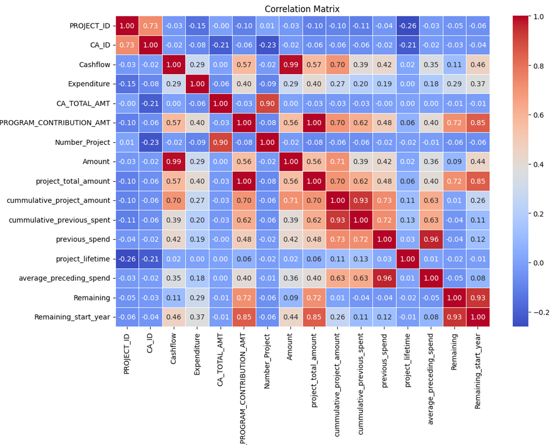
Figure 3: Correlation Matrix – overview of multicollinearity among variables
The correlation matrix provides an overview of the relationships between all variables in the model. Each cell represents the correlation coefficient between two variables, ranging from -1 (strong negative correlation) to 1 (strong positive correlation). Highly correlated variables indicate potential redundancy, while weak or no correlation suggests independent features. The diagonal values are always 1, as each variable is perfectly correlated with itself. This matrix helps in identifying multicollinearity, selecting the most relevant features, and understanding variable interactions within the dataset.
By applying PCA, we transformed the original features into orthogonal components, capturing the maximum variance in a reduced-dimensional space. The explained variance analysis showed that five components retained about 90% of the total variance, preserving most of the dataset's information while reducing dimensionality. This trade-off mitigates multicollinearity while maintaining the predictive power of key features.
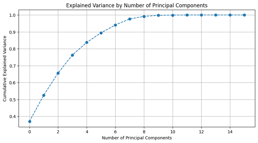
Figure 4: Variance by number of component
The graph illustrates the explained variance as a function of the number of principal components (PCs). The curve shows a steep increase at the beginning, indicating that the first few components capture most of the variance in the dataset. With five principal components, the cumulative explained variance reaches 90%, suggesting that these components retain most of the essential information while reducing dimensionality. Beyond this point, additional components contribute marginally to the total variance, emphasizing the effectiveness of using five PCs for data representation.
The PCA was used to reduce multicollinearity among the financial variables while preserving the most informative features. Figure 5: PCA results illustrates this method loadings, which represent how strongly each original variable contributes to a given principal component.
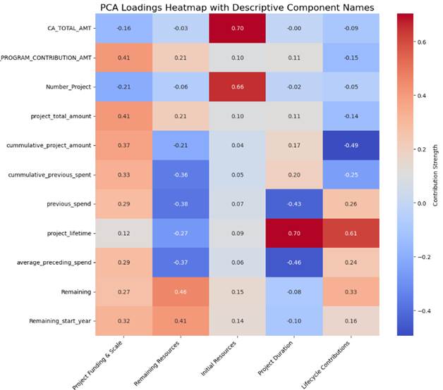
Figure 5: PCA results
The PCA loadings heatmap visually represents the contribution of each original variable to the principal components, highlighting key dimensions of project expenditures. Each principal component was derived to encapsulate a distinct financial aspect of the projects. Project Funding & Scale is primarily influenced by the total program contribution amount, project total amount, and cumulative project amount, reflecting the overall financial scope. Remaining Resources captures unspent funds, dominated by variables related to remaining budget values. Initial Resources focuses on the initial financial allocation, showing moderate contributions from total program contributions and project total amounts. Project Duration is strongly associated with project lifetime, indicating its role in capturing time-related aspects. Lastly, Lifecycle Contributions represents historical spending trends through variables such as cumulative project amount, previous spend, and average preceding spend. This dimensionality reduction approach mitigates multicollinearity, ensuring the model remains stable while preserving the explanatory power of financial predictors.
To improve interpretability, the principal components were renamed based on their dominant loadings:
- Principal Component 1: Project Funding & Scale – This component is influenced by TOTAL_PROGRAM_CONTRIBUTION_AMT (0.41), project_total_amount (0.41), and cumulative_project_amount (0.37). It represents the overall financial scale of a project, emphasizing the total funding available.
- Principal Component 2: Remaining Resources – This component captures the availability of unspent funds, primarily driven by Remaining (0.46) and Remaining_start_year (0.41). It indicates the funding is still accessible for ongoing projects.
- Principal Component 3: Initial Resources – This component is moderately influenced by TOTAL_PROGRAM_CONTRIBUTION_AMT (0.21), project_total_amount (0.10), and cumulative_project_amount (0.04), suggesting it relates to the initial allocation of financial resources at the start of a project.
- Principal Component 4: Project Duration – This component strongly correlates with project_lifetime (0.70), indicating that it captures project longevity and its relationship to past spending trends.
- Principal Component 5: Lifecycle Contributions – This component captures the financial balance across a project’s timeline, with strong contributions from project_lifetime (0.61) and previous_spend (0.26).
By integrating PCA into our modeling pipeline, we effectively addressed the collinearity issues present in the original dataset and improved the stability and interpretability of the model.
The review also highlighted an important consideration: if most of the variance is not captured within a few components, it may indicate a complex data structure or non-linear relationships. In such cases, techniques like Kernel PCA, t-SNE, or UMAP might be more suitable. However, since PCA with five components retains 90% of the variance, it remains a valid choice for dimensionality reduction in this context. Future work could further explore non-linear embeddings to determine if an alternative approach provides additional performance gains.
4. G&Cs Machine Learning Forecasting Model Development
With the pre-processing complete, the next phase focused on building a robust forecasting model. This involved selecting an appropriate algorithm, fine-tuning hyperparameters, and evaluating performance to ensure accuracy across diverse project scales. Given the complexity of financial data, our approach prioritized interpretability, stability, and alignment with business needs.
4.1. Final Dataset
| Variable | Definition | Sample Data |
|---|---|---|
| Project ID | A unique identifier for each project | 13176 |
| Contribution Agreement ID | A unique identifier linking the project to a specific funding agreement. | 2 |
| Fiscal Year | The fiscal year associated with the project’s expenditures and cashflows. | 2007-2008 |
| Project Cashflow | The projected or actual cash inflow and outflow for the project. | 500 000 |
| Project Expenditure | The amount spent on the project within a given period. | 500 000 |
| Total Amount per Contribution Agreement | The full allocated budget under a specific agreement. | 2 000 000 |
| Project Status | Indicates the current state of the project (e.g., active, completed, pending). | Closed |
| Amount | A derived variable used to improve forecast accuracy. Target variable. | 500 000 |
| PC1 | Project funding & scale: It represents the overall financial scale of a project, emphasizing the total funding available. | -0.68 |
| PC2 | Remaining resources: It indicates the funding is still accessible for ongoing projects. | 0.97 |
| PC3 | Initial resources: it relates to the initial allocation of financial resources at the start of a project. | -1.34 |
| PC4 | Project Duration: it captures project longevity and its relationship to past spending trends. | -0.19 |
| PC5 | Lifetime Contribution: captures the financial balance across a project’s timeline, with strong contributions from project_lifetime and previous_spend | -0.08 |
Note: As segmentation was part of the test scenarios, we initially maintained two separate datasets—df_high and df_low—grouping projects based on their materiality level.
4.2. Model Training
The dataset was structured as a time series, covering fiscal years from 2003-2004 up to 2023-2024. It was split into a training set (75%) and a test set (25%), ensuring that past data was used to forecast future expenditures. Once trained, the model was applied to predict expenditures for the current fiscal year (2024-2025) and projected three years into the future. The training process was iterative, refining the models to optimize performance while maintaining stability.
4.3. Model Comparison
Several models were evaluated, including Random Forest, Gradient Boosting, and XGBoost, based on their predictive accuracy and ability to capture patterns in financial data. Since expenditures follow a sequential pattern over time, the models needed to account for temporal dependencies and underlying trends.
Each model had distinct characteristics:
- Random Forest, an ensemble method, effectively captured complex interactions, making it a strong candidate for financial forecasting.
- Gradient Boosting refined predictions through iterative learning, improving accuracy.
- XGBoost, an optimized gradient boosting algorithm, enhanced accuracy further and addressed overfitting concerns.
Model performance was evaluated using two key metrics:
- R² (Coefficient of Determination): Measures how well the model explains variance in expenditures.
- MAE (Mean Absolute Error): Quantifies the average prediction error, providing a clear financial accuracy measure.
4.4. Model Performance Assessment
This section presents the assessment metrics used to compare different models. The objective was to balance predictive accuracy, stability, and interpretability while capturing the complexities of financial data.
| Scenarios | Characteristics | Best Model Performance (metrics) |
|---|---|---|
| Scenario 1 |
|
Random Forest (MAE: 137,570; R²: 93%) Overfit |
| Scenario 2 |
|
Random Forest (MAE: 852,243; R²: 36%) |
| Scenario 3 |
|
Random Forest (MAE: 888,558; R²: 37%) |
| Scenario 4 |
|
Random Forest (MAE: 888,526; R²: 81%) |
| Scenario 5 |
|
Random Forest (MAE: 758,012; R²: 40%) |
4.5. Model Performance Assessment Consideration
To optimize model performance, various test splits were evaluated, including both 25%-30% and automated splits. Each scenario was tested to assess how different training and testing data partitions impacted the model's accuracy and generalizability. The automated split approach was also considered, ensuring the model’s performance remained robust across different data partitioning strategies. This comprehensive testing allowed for the identification of the most effective split configuration to enhance the model's predictive capabilities.
After optimizing the test split, we evaluated the impact of segmentation and PCA on model performance. While segmentation was initially expected to improve accuracy, testing showed that removing it while retaining PCA resulted in more stable and precise forecasts. Initially, segmentation led to the creation of two separate datasets, grouping projects based on predefined criteria. However, further analysis revealed that a unified dataset provided greater consistency, simplified model implementation, and improved scalability. This finding underscored the effectiveness of dimensionality reduction in capturing key patterns while minimizing noise. Consequently, PCA was prioritized as the primary technique for managing data complexity, ensuring a more robust and generalizable forecasting model.
Finally, we conducted hyperparameter tuning using both manual adjustments and automated optimization. However, tuning did not always yield significant improvements. For instance, a tuned Random Forest model achieved a slightly lower MAE (811,547) and a higher R² (39%), but this marginal gain did not justify the increased complexity. In some cases, hyperparameter tuning introduced overfitting, reinforcing the reliability of the simpler, default configuration.
4.6. Best Model Results
Our analysis revealed that Random Forest consistently outperformed other models in balancing predictive accuracy and alignment with financial forecasts. Among the tested configurations, the best-performing model was Random Forest (MAE: 852,243, R²: 36%), which provided expenditure projections of 4.8B for 2024-2025 and 5.2B for 2025-2026, making it the closest to GCCOE predictions. The formula for accuracy is:
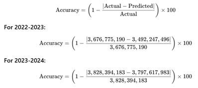
Figure 6: Accuracy computation
The ML model demonstrated an accuracy rate of 94,98% and 99,20% for fiscal years 2021-22 and 2022-23 respectively. The degree of accuracy is promising and has led to the models' implementation by FMAs as part of their process for forecasting expenditures for fiscal years 2024-25 to 2026-27.
4.7. ML Forecast Model Limitations
Despite the promising results, there are several limitations to the ML forecasting model that need to be addressed. Programs without project records in the system cannot be modeled because the model needs to know a project exists to generate a forecast for it. In addition, the model was created to forecast reimbursement-based claims for direct delivery programs. As such, it is less accurate when it comes to forecasting for other types of payments such as grants, advances, and milestone-based claims. The model is also less accurate for allocation-based or flow through G&C programs. Lastly, the model’s accuracy diminishes at the individual project level, which can exhibit atypical spending patterns.
These limitations mean the model currently performs best for direct delivery programs with 30 or more active projects in the system and for which the majority of claims are reimbursement based.
5. Business Results
5.1. How to get ML in the hands of the business:
To enhance the interpretation of the model's results, forecasted expenditures were integrated into an existing dashboard used by FMAs (Figure 7). This dashboard visually represents expenditure trends, allowing comparisons between actual expenditures, the FMAs' current manual method, and the ML model's forecasts.
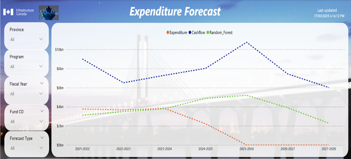
Figure 7: PowerBI Results Visualization
This screenshot is for illustration purposes only and does not contain real HICC data. It features a line chart where the orange line represents expenditures, the blue line represents cash flow, and the green line represents the Random Forest forecast, helping visualize historical trends and future projections. Below the chart, a data table provides project-level details, allowing deeper analysis. On the left, a filter panel enables FMA to refine their research by selecting specific criteria, ensuring a focused and customized view of the data. Both the chart and table dynamically adjust based on these filters, enhancing usability and insight generation.
The interactive dashboard also features personalized report capabilities, allowing users to customize their views by selecting specific criteria, such as province, program, and fiscal year. This flexibility ensures that users can tailor the data exploration to meet their specific analytical needs. Furthermore, the interactive nature of the visualization allows users to hover over any point on the curves to view exact values for each fiscal year, offering a more intuitive and granular exploration of the data. This combination of dynamic reporting and interactive visualizations supports in-depth analysis and facilitates decision-making based on the ML model's output.
5.2. Business Impact
The ML model was implemented in May 2024 to forecast G&C spending for fiscal years 2024-25 through 2027-28. It generated multi-year forecasts for nine of the department’s G&C programs, which account for approximately 80% of the department’s Grants and Contributions funding. The model's accuracy will be evaluated in April 2025 and April 2026, at the close of fiscal years 2024-25 and 2025-26, respectively.
The model’s implementation streamlined the forecasting process, reducing the time required from three months to one month. This was achieved by providing FMAs with a baseline forecast – generated by the ML model – which facilitated discussions with their respective programs and aligned expectations ahead of the recipient cash flow collection process.
Additionally, the integrated dashboard supports ongoing discussions with stakeholders, using up-to-date data in preparation for regular departmental reporting.
6. Conclusion and Next Steps
In conclusion, this study highlights the significant potential of the implementation of a ML forecasting model in the context of expenditure prediction for HICC G&C programs. The model demonstrates a high level of accuracy when compared against historic expenditures and is being tested against actual expenditures over the next two years in hopes of optimizing Grants and Contributions funding, reducing public account lapses, and streamlining financial processes. Despite the challenges and limitations mentioned, the overall results have shown promise in enhancing financial decision-making and operational efficiency.
The success of this initiative was formally recognized in December 2024 when the project received the 2024 Controller General Innovation Award, recognizing its significant impact in financial management. Since then, the model has garnered attention across various government departments, prompting consultations to explore its broader application. The ongoing efforts to promote its adoption reflect a growing recognition of the potential for ML-driven solutions to improve financial forecasting and resource allocation across the public sector.
Additionally, the project was longlisted for the 2025-2026 edition of the Public Service Data Challenge. This recognition highlights the increasing interest and enthusiasm from multiple departments to adopt the ML-driven forecasting tool. Ongoing efforts to promote its adoption further underscore the growing recognition of the potential for machine learning solutions to enhance financial forecasting and optimize resource allocation across the public sector.
Subscribe to the Data Science Network for the Federal Public Service newsletter to keep up with the latest data science news.