
Greenhouse Detection with Remote Sensing and Machine Learning: Phase One
By: Stan Hatko, Statistics Canada
A modernization effort is underway at Statistics Canada to replace agricultural surveys with more innovative data collection methods. A key part of this modernization is the use of remote sensing classification methods of land use mapping and building detection from satellite imagery.
Currently, Statistics Canada conducts the Census of Agriculture every five years to collect information on topics such as population, yields, technology and agricultural greenhouse use in Canada. Data scientists have been teaming up with subject matter experts to modernize the collection of these data, as traditional methods are not sustainable in the long term. Innovative methods are needed to ensure the agency can continue to produce new information for the agriculture sector in an efficient manner. This project will allow the agency to make data available in a more timely manner and reduce the response burden for agricultural operators.
This project explores the machine learning techniques used to detect the total area of greenhouses in Canada from satellite imagery.
Satellite imagery
This project used RapidEye satellite images which have 5-metre pixel resolution (that is, each pixel is a 5 m by 5 m square) with 5 spectral bands.
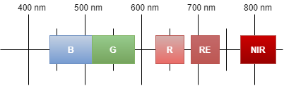
Description for Figure 1 - Graphical representation of spectral bands for RapidEye satellite imagery
A graphical representation of the spectral range of each band in a RapidEye output image: (1) blue (440 – 510 nm), (2) green (520 – 590 nm), (3) red (630 – 685 nm), (4) red edge (690 – 730 nm), and (5) near infrared (760 – 850 nm).
This imagery was chosen due to its relative availability and cost. Lower resolution imagery is not always adequate to detect greenhouses, and higher resolution imagery would have proven prohibitively expensive given the total area required to cover the Canadian agricultural sector.
Labelled shape data
For certain sites the subject matter experts labelled data in the form of Shapefiles indicating which areas correspond to greenhouses. This was done manually by looking at extremely high resolution satellite and aerial imagery (using Google Earth Pro and similar software), and highlighting the area corresponding to greenhouses.
These labelled data had two roles:
- Training data (from certain sites) to build a machine learning classifier to determine the area covered by greenhouses.
- Testing data (from other sites) to evaluate the performance of the classifier.
Labelled data from Leamington, Ontario; Niagara, Ontario; and Fraser Valley, British Columbia were produced. Certain sites were chosen as training sites (like Leamington West), while others were chosen to be testing sites (like Leamington East).
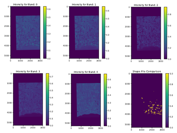
Figure 2 is an example of RapidEye imagery of a region together with the greenhouse labelling file.
 .
.
Description for Figure 2 - The five spectral bands and greenhouse indicator based on Shapefiles for one area of interest
A comparison of each of the five spectral bands against the Shapefiles of labelled greenhouses.
The labelled data were broken down into sites and sub-sites to train and validate the machine learning model. The training sites were:
- Leamington West
- Niagara North: N1, N1a, N3
- Fraser South: S1, S2, S3, S4, S5
Validation sites were used to test the model were:
- Leamington East
- Niagara South: S1, S2
- Fraser North: N2, N3, N5
Machine learning methodology
For each point, the data scientists needed to predict if it corresponded to a greenhouse or not, as well as a predicted probability of each point being a greenhouse.
For prediction, given a point, a window of specified size was taken around the point. This was fed in the data in this window to the classifier, which attempted to then predict if the central point is a greenhouse or not. The window around the point provided additional context to help the classifier determine if the central point is a greenhouse or not.
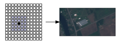
Description for Figure 3 - The classifier
A grid representing an input window that evaluates pixels in a source image to try and classify them as greenhouses or not.
The classifier needs to determine if the central dark point corresponds to a greenhouse, based on the highlighted area around that point.
This process was repeated for every point in the image (except near borders), and resulted in a map showing the exact area covered by greenhouses.
For training, a sample of many such points (with the window around each point) was taken and fed in (with the label) to construct the model. The training set size was also increased by applying various transformations, for instance rotating the input image by different angles for different points.
Initial work and transition to cloud
Originally the work was done on a Statistics Canada internal system with 8 CPU cores and 16 GB of RAM. Several algorithms were tested for the classifier, including support vector machines, random forests, multilayer perceptron, and multilayer perceptron with principal component analysis (PCA).
The best results were obtained with PCA and multilayer perceptron, resulting in an F1 Score of 0.89 to 0.90 for Leamington East. Various system limitations were reached during this work, such as a lack of a dedicated Graphics Processing Unit (GPU). The GPU is required to efficiently train more complex models involving convolutional neural networks.
The public cloud was explored as an option as there were no sensitive data for this project. The project was transferred to the Microsoft Azure cloud, on a system with 112 GB of RAM, large amounts of storage and a very powerful NVIDIA V100 GPU. The Microsoft Azure Storage Explorer software was used to transfer data to and from the storage account.
Convolutional neural networks
Convolutional neural networks (ConvNets) incorporate the concepts of locality (neighbourhood around point in image being important) and translation invariance (same features useful everywhere) into a neural network. Architectures based on this have been considered state-of-the-art in image recognition for several years.
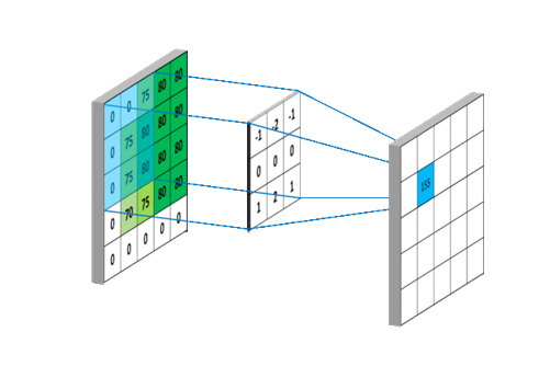
A layer in a basic ConvNet works as follows:
- Around each point in the image or previous layer, a small window (for instance, 3x3) is taken.
- The data in that window are multiplied by a matrix, to which the activation is applied (a bias can be added as well).
- This process is repeated for every point in the image (or previous layer), to obtain the new layer. The same matrix is used each time.
This equivalently corresponds to multiplying by a large sparse matrix, with certain weights tied to same values, followed by the activation.
Many different architectures based on ConvNets are possible. This project tested the following options:
- Simple ConvNet: Apply convolutional layers in sequence (output of layer is input to next), followed by fully connected.
- ResNet: Apply convolutional layer with same size output, and add to original (so input of next layer is sum of original and this layer). Can repeat this for many layers. Has been used to train extremely deep networks.
- DenseNet: Apply convolutional layer, and append outputs to original as new channels. Each layer adds new channels, which can be useful features.
- Custom branched architecture: Crop central part of window, and apply one convolutional network. Take the whole image, and apply another network (with more dimensionality reduction based on pooling layers). Merge both at the end in fully connected layer. This allows the user to focus in on the part near the central point, while getting some context around it.
The data scientists used the custom branched architecture for this project, as shown in figure 5.

Description for Figure 5 - Diagram of the convolutional neural network architecture chosen for this project
- The input has a window size of 10 around the central point (square of size 21 x 21), with the 5 spectral bands from RapidEye.
- A convolutional layer with 64 filters, kernel size 3, and stride 1 is applied. Batch normalization is applied, followed by the ReLU (rectified linear unit) nonlinearity.
- The output of the above is then split into two parts, one that focuses on the central region and one that considers a larger context window with down sampling.
- For the first path (the ‘focus' path), the following is performed:
- A window of size 5 around the central point is taken, and that part is subsetted (an 11 x 11 square centered around the central point).
- A convolutional layer with 64 filters, kernel size 3, and stride 1 is applied. This is followed by batch normalization and the ReLU nonlinearity.
- A convolutional layer with 64 filters, kernel size 3, and stride 1 is applied. This is followed by batch normalization and the ReLU nonlinearity.
- For the second path (the ‘surround' path), the following is performed:
- A convolutional layer with 64 filters, kernel size 3, and stride 1 is applied. This is followed by batch normalization and the ReLU nonlinearity.
- Max-pooling of size 2 is applied.
- A convolutional layer with 64 filters, kernel size 3, and stride 1 is applied. This is followed by batch normalization and the ReLU nonlinearity.
- The output for both of the above paths is flattened and concatenated.
- A dense layer with 128 units is applied, followed by batch normalization and the ReLU nonlinearity.
- A dense layer with 64 units is applied, followed by batch normalization and the ReLU nonlinearity.
- The output layer with a single linear output is used, followed by the sigmoid function to produce a probability.
- For prediction, the above output is used as-is for the predicted probability of the point being a solar panel. A threshold of 0.5 is used for discrete prediction (if greater than 0.5, is a greenhouse, otherwise not a greenhouse). For training, the binary cross entropy loss is used with the above as the predicted value and the shapefile label as the ground truth label.
For optimization, the ADAM optimizer was used with a learning rate of 10-5. A mini-batch size of 5,000 was used, and the training was done for 50 epochs.
Results
After the model was trained, it was tested on each of the validation sites in Leamington East, Niagara South, and Fraser North. The results are summarized in the table below.
| Region | Leamington East | Fraser N2 | Fraser N3 | Fraser N5 | Niagara S1 | Niagara S2 |
|---|---|---|---|---|---|---|
| Count Unknown | 338443 | 292149 | 292149 | 246299 | 388479 | 388479 |
| Count True Negative (TN) | 14320042 | 12347479 | 12350813 | 8608499 | 24597241 | 24598805 |
| Count False Positive (FP) | 9984 | 1069 | 1875 | 2337 | 2143 | 2411 |
| Count False Negative (FN) | 6880 | 957 | 1069 | 5474 | 3248 | 1049 |
| Count True Positive (TP) | 138315 | 8346 | 4094 | 5041 | 8889 | 9256 |
| Accuracy | 0.998835 | 0.999836 | 0.999762 | 0.999094 | 0.999781 | 0.999859 |
| Precision | 0.932677 | 0.886458 | 0.685877 | 0.683247 | 0.805747 | 0.793349 |
| Recall | 0.952615 | 0.89713 | 0.79295 | 0.47941 | 0.732389 | 0.898205 |
| F1 | 0.942541 | 0.891762 | 0.735537 | 0.563461 | 0.767318 | 0.842527 |
| AUROC | 0.999508 | 0.999728 | 0.998477 | 0.962959 | 0.977933 | 0.999949 |
For Leamington, the result obtained was very good: the greenhouses were picked up well and false positives were small. The number of misclassified points (FP and FN) was much smaller than both the correct classes (TN and TP). This area has the best overall F1 score at slightly over 0.94.
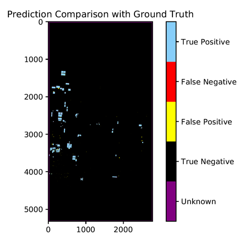
Description for Figure 6 - Leamington East Results
A spatial representation of the classification of detected items as True Positive, True Negative, False Positive, False Negative, or unknown.For Niagara, the results were generally good: most of the greenhouse area was predicted correctly. There was a false positive greenhouse below left of the detected greenhouses in Niagara S1 (Figure 7). This corresponds to a river-coastal area. Originally this false positive was significantly larger, but increasing the sample size for a coastal urban area (with a fairly straight coastline) significantly reduced the size and also helped with some other areas. If more coastline images were added to the training set (with different river beds, etc.) this error may be further reduced.
Description for Figure 7 - Niagara S1 greenhouse results
A spatial representation of the classification of detected items as True Positive, True Negative, False Positive, False Negative, or unknown.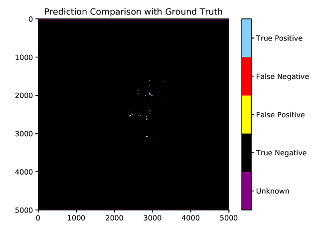
Description for Figure 8 - Niagara S2 greenhouse results
A spatial representation of the classification of detected items as True Positive, True Negative, False Positive, False Negative, or unknown.For Fraser, the results varied depending on the area. For Fraser N2 (Figure 9) the results were good. The results were not as good for Fraser N3 (Figure 10), as a cluster of small greenhouses right of the detected greenhouses were missed (along with some false positives). For Fraser N5 (Figure 11) a significant number of greenhouses were missed. Various experimentation so far has not improved the results for Fraser. To improve these results, the team would need to investigate what type of greenhouses these are, if additional areas containing these types of greenhouses can be added to the training set, and even if this type of greenhouse can be detected from the 5m satellite images.
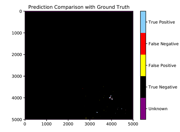
Description for Figure 9 - Fraser N2 greenhouse results
A spatial representation of the classification of detected items as True Positive, True Negative, False Positive, False Negative, or unknown.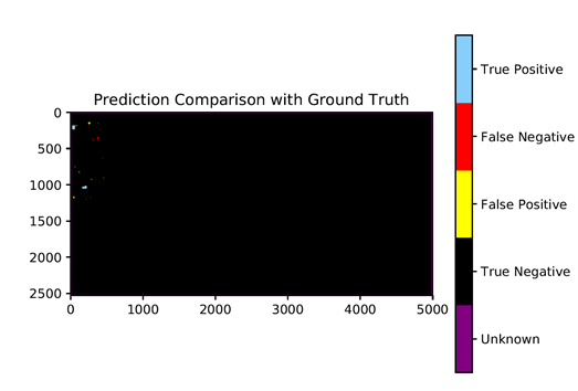
Description for Figure 10 - Fraser N3 greenhouse results
A spatial representation of the classification of detected items as True Positive, True Negative, False Positive, False Negative, or unknown.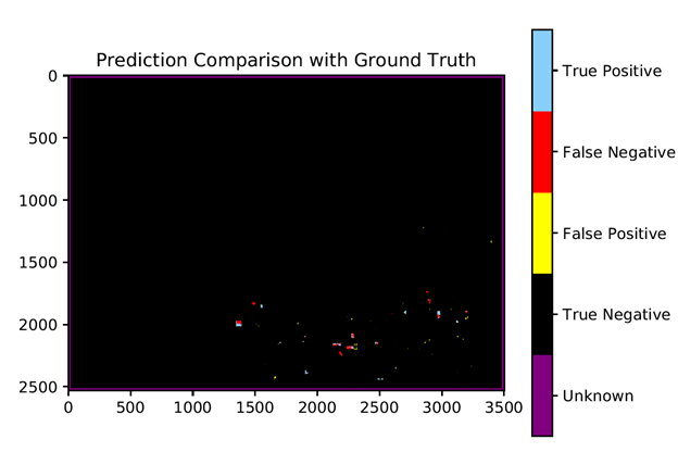
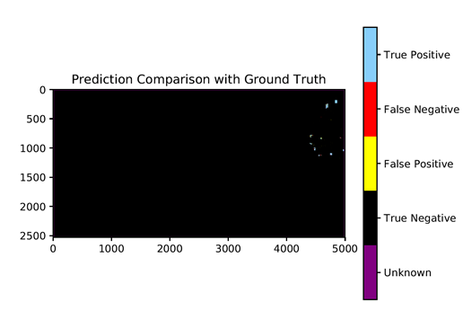
Description for Figure 11 - Fraser N5 greenhouse result
A spatial representation of the classification of detected items as True Positive, True Negative, False Positive, False Negative, or unknown.Conclusion
Overall, convolutional neural networks were successfully used to detect greenhouses from satellite images in multiple areas. This was particularly true in the areas of Leamington, Niagara, and Fraser. Other areas are still showing low prediction levels for greenhouses. Additionally, there are still issues with small greenhouses in all three areas of interest, which were not large enough to be detected in the 5m RapidEye satellite imagery. These challenges could be solved by higher resolution aerial acquisitions.
The next phase of this project will explore greenhouse detection from higher resolution aerial images. Different methodologies are used when working with higher resolution aerial imagery, for instance the use of UNet-based image segmentation architectures to identify areas corresponding to greenhouses, which we look forward to exploring in a future article.
- Date modified: