
Topic Modelling and Dynamic Topic Modelling : A technical review
By: Loic Muhirwa, Statistics Canada
In the machine learning subfield of Natural Language Processing (NLP), a topic model is a type of unsupervised model that is used to uncover abstract topics within a corpus. Topic modelling can be thought of as a sort of soft clustering of documents within a corpus. Dynamic topic modelling refers to the introduction of a temporal dimension into a topic modelling analysis. The dynamic aspect of topic modelling is a growing area of research and has seen many applications, including semantic time-series analysis, unsupervised document classification, and event detection. In the event detection case, if the semantic structure of a corpus represents real world phenomenon, a significant change in that semantic structure can be used to represent and detect real world events. To that end, this article presents the technical aspects of a novel Bayesian dynamic topic modelling approach in the context of event detection problems.
A proof-of-concept dynamic topic modelling system has been designed, implemented and deployed using the Canadian Coroner and Medical Examiner Database (CCMED), a new database developed at Statistics Canada in collaboration with the 13 provincial and territorial Chief Coroners, Chief Medical Examiners and the Public Health Agency of Canada. The CCMED contains standardized information on the circumstances surrounding deaths reported to coroners and medical examiners in Canada. In particular, the CCMED contains unstructured data in the form of free-text variables, called narratives, that provide detailed information on the circumstances surrounding these reported deaths. The collection of the narratives forms a corpus (a collection of documents) that is suitable for text-mining and so the question follows: can machine learning (ML) techniques be used to uncover useful and novel hidden semantic structures? And if so, can these semantic structures be analyzed dynamically (over time) to detect emerging death narratives?
The initial results look promising and the next step is twofold: firstly, further fine-tuning of the system and construction of event detections. Secondly, since this system will be used as an aid for analysts to study and investigate the CCMED, the insights coming out of the system will need to be aligned with human interpretability. This article gives a technical overview of the methodology behind topic modelling, explaining the basis of Latent Dirichlet Allocation and introducing a temporal dimension into the topic modelling analysis. A future article will showcase the application of these techniques on the CCMED.
Latent Dirichlet Allocation
Latent Dirichlet Allocation (LDA)Footnote 1 is an example of a topic model commonly used in the ML community. Due to the performance of LDA models, it has several production-level implementations in popular data-oriented scripting languages like PythonFootnote 2. LDA was first introduced as a generalization to Probabilistic Latent Semantic Analysis (PLSA)Footnote 3 presenting significant improvements; one of them being fully generativeFootnote 4.
The model
LDA is regarded as a generative model as the joint distribution (likelihood-prior product) is explicitly defined; this allows documents to be generated by simply sampling from the distribution. The model assumptions are made clear by examining the generative process that describes how each word in a given document is generated.
Put formally, suppose are the number topics and the size of our entire vocabulary respectively. The vocabulary refers to the set of all terms used to generate the documents. Furthermore, suppose that and are vectors representing discrete distributions over topics and vocabulary respectively. In LDA a document is represented by a distinct topic distribution and a topic is represented by a distinct word distribution. Let be a one-hot vector representing a particular word in the vocabulary and let be a one-hot vector representing a particular topic.
The notation and can be used to describe the generative process that generates a word in a document by sampling a topic distribution and a word distribution. LDA assumes that these distributions are drawn from Dirichlet distributions, that is and where and are the sparsity parameters. Then using those distributions, first draw a topic assignment and then from that topic draw a word . In other words, the words within a document are sampled from a word distribution governed by a fixed topic distribution representing that document. Figure 1 demonstrates this generative process in graphical plate notation, for a corpus of size with documents of a fixed size . Though the document size is usually assumed to come from an independent Poisson process, for now, to simplify the notation, it is assumed without loss of generality, that the documents have a fixed size.
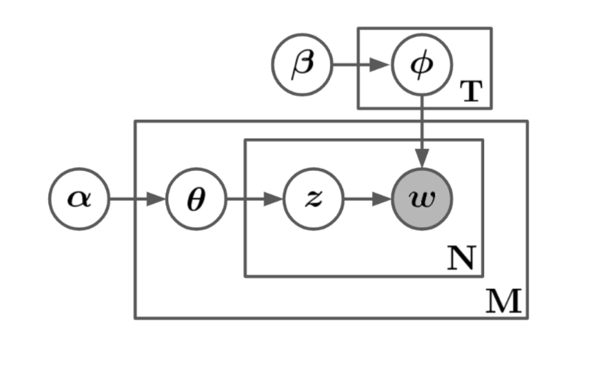
Description Figure 1 - Plate notation of the generative process. The boxes are “plates” representing replicates and shaded nodes are observed.
An illustration of the LDA generative process in plate notation. The diagram is composed of a directed acyclic graph, where the nodes represent variables and the edges represent variable dependencies. The outermost nodes of the directed graph are the model hyperparameters and these nodes have no in-edges, meaning they do not depend on any other parameter of the model. From the hyperparameters, edges lead into the other variables until they reach a final node, representing a word. From one end, the topic hyperparameter node, leads into a word distribution node, which finally leads into the word node. From another endpoint, the document hyperparameter, leads into a topic distribution node, which leads into a word-topic assignment node and then finally the word node. This word node is shaded and is the only node that is shaded, the shading indicates that the node in question represents an observed variable; implying that every other node in the graph is unobserved. Some nodes are enclosed in a rectangular box with a variable at the bottom-right corner of the box. The boxes represent repetitions and the bottom-right variable represents the size of that repetition. The word distribution node is enclosed in a box with a variable number of repetitions, T. The word-topic assignment and word nodes are enclosed in a box with a variable number of repetitions, N. This previous box is further enclosed into a larger box that includes the topic distribution node a variable number of repetitions, M. Since the word-topic assignment and word nodes are enclosed in two boxes, those two variables have a number of repetitions that is equal to the product of the variable at the bottom-right corner of the two boxes, in this case, N times M.
| Variable | Description |
|---|---|
| A set representing all raw documents, i.e., the corpus | |
| Number of topics | |
| Number of words in the vocabulary | |
| Topic distribution representing the document; this is an dense vector | |
| Word count in the document | |
| Word distribution representing the topic; this is an dense vector | |
| Topic assignment for the word in the document; this is an one-hot vector | |
| Vocabulary assignment for the word in the document; this is an one-hot vector | |
| Dirichlet sparsity parameter for topics | |
| Dirichlet sparsity parameter for documents |
Let be a set representing the collection of all topic assignments, this is a set of size and let be a set representing the collection of all topic distributions (documents) and finally, let be a random matrix representing the collection of all word distributions (topics), i.e., . It follows that if the entry in a given topic assigned, say is 1 then:
Equation 1:
Following the notation from above, the joint distribution can be defined as follows:
Equation 2:
Since one of the model assumptions is that the topic distributions are conditionally independent on β, the following form is equivalent:
Equation 3:
Now that the model is specified, the generative process might seem clearer in pseudo-code. Following the joint distribution, the generative process goes as follows:
Given: V, T,
for do
end for
for do
for do
end for
end for
It is worth pointing out that T, the number of topics, is fixed and being fixed is indeed a model assumption and requirement—this also implies, in the Bayesian setting, that T is a model parameter and not a latent variable. This difference is far from trivial, as shown in the inference section.
It is important to distinguish LDA from a simple Dirichlet-multinomial clustering model. A Dirichlet-multinomial clustering model would involve a two-level model in which a Dirichlet is sampled once for a corpus, a multinomial clustering variable is selected once for each document in the corpus, and a set of words is selected for the document conditional on the cluster variable. As with many clustering models, such a model restricts a document to being associated with a single topic. LDA, on the other hand, involves three levels, and notably, the topic node is sampled repeatedly within the document. Under this model, documents can be associated with multiple topicsFootnote 1.
Inference
Inference with LDA amounts to reverse-engineering of the generative process described in the previous section. As the generative process goes from topic to word, the posterior inference will therefore go from word to topic. With LDA we assume that and are latent variables rather than model parameters. This difference has a drastic impact on the way the quantities of interest are inferred, which are the distributions and . In contrast, if and were modelled as parameters the Expectation Maximization (EM) algorithm could be used to find the maximum likelihood estimate (MLE). After the convergence of the EM algorithm, it retrieves the learned parameters to accomplish the goal of finding the abstract topics within the corpus. EM provides point estimates of the model parameter by marginalizing out the latent variables. The issues here are that the quantities of interest are being marginalized out and the point estimation wouldn't be faithful to the Bayesian inference approach. For a true Bayesian inference, access to the posterior distribution of the latent variables , and would be needed. Next, this posterior distribution is examined and some computational difficulties which will help motivate an inference approach will be pointed out.
The posterior has the following form:
Equation 4:
A closer look at the denominator:
Equation 5:
Equation (5) is known as the evidence and acts as a normalizing constant. Calculating the evidence requires computing a high dimensional integral over the joint probability. As shown in equation (5), the coupling of and makes them inseparable in the summation and thus this integral is at least exponential in , making it intractable. The intractability of the evidence integral is a common problem in Bayesian inference and is known as the Inference ProblemFootnote 1. LDA inference and implementations differ in the way they overcome this problem.
Variational inference
In modern machine learning, variational (Bayesian) inference (VI), is most often used to infer the conditional distribution over the latent variables given the observations and parameters. This is also known as the posterior distribution over the latent variables (equation (2)). At a high level, VI is straightforward: the goal is to approximate the intractable posterior with a distribution that comes from a family of tractable distributions. This family of tractable distributions are called variational distributions (from variational calculus). Once the family of distributions are specified one approximates the posterior by finding the variational distribution that optimizes some metric between itself and the posterior. A common metric used to measure the similarity between two distributions is the Kullback-Leibler divergence and it is defined as follows: divergence and it is defined as follows:
Equation 6: \
Where and are probability distributions over the same support. In the original LDA paperFootnote 1 the authors propose a family of distributions having the following form:
Equation 7:
Where , and are free variational parameters. This family of distributions is obtained by decoupling and (this coupling is what led to intractability), which makes the latent variables conditionally independent on the variational parameters. Thus, the approximate inference is reduced to the following deterministic optimization problem:
Equation 8:
Where is the posterior of interest and its final approximation is given by:
Equation 9:
In the context of the problem, the optimization problem in equation (8) is ill-posed since it requires and approximating is the original inference problem. It is straightforward to show the following:
Equation 10:
Equation 11:
is called the Evidence Lower Bound (ELBO) and though it depends on the likelihood it is free of and therefore tractable. Therefore, the optimization problem in equation (8) is equivalent to the following optimization problem:
Equation 12:
Thus, inference in LDA maximizes the ELBO over a tractable family of distributions to approximate the posterior. Typically, a stochastic optimization approach is implemented to overcome the computational complexity—stochastic coordinate descent in particular. Further details on the analysis of VI is provided inFootnote 1, sections 5.2, 5.3, and 5.4 ofFootnote 1, and section 4 ofFootnote 4.
Dynamic topic modelling
Dynamic topic modelling refers to the introduction of a temporal dimension into the topic modelling analysis. In particular, dynamic topic modelling in the context of this project, refers to studying the change over time of specific topics. The project aims to analyze fixed topics over a particular time interval. Since the documents coming out of the CCMED have a natural time stamp, the date of death (DOD), they provide a canonical way to split the complete dataset into corpora covering a specific time interval. Once the data are split, the LDA can be applied to each individual corpus and then it is possible to analyze how each topic evolves over time.
One challenge with this dynamic approach is mapping the topics from two adjacent time windows. Because of the stochastic nature of the optimization problem in the inference stage, every time an instance of LDA is run, the ordering of the resulting abstract topics is random. Specifically, given two adjacent time windows indexed by and and a fixed topic indexed by , how can it be assured that the topic at time corresponds to the topic at time ? To answer this, it is possible to construct topic priors for time by using learned topic parameters from time . To have a better understanding of the mechanism, the term prior refers to the parameters of the prior distributions and not the distributions themselves; equivalently this refers to quantities that are proportional to the location (expectation) of the prior distributions. Under this setting, the topic prior can be represented by a matrix such that the entry is the prior on the term given the topic. Note that without any prior information or domain knowledge about , the probability parameter of the term given the topic, a uniform prior would be imposed by making a constant and therefore it would be minimally represented by a scalar. Whenever is constant, the resulting Dirichlet distribution is symmetric and it is said to have a symmetric prior, which is the constant. Suppose that at time we learned topic parameter matrix , before learning we will impose a prior with the following form:
Equation 13:
Matrix serves as an informative prior for , essentially implying that it is assumed that the topic distributions from adjacent time windows are similar in some sense. serves as an uninformative uniform prior, this matrix essentially smooths out the sharp information from . Keeping in mind that the vocabulary also evolves over time, meaning that some words are being added and some words are being removed from the vocabulary as the model sees new corpora, meaning this has to be accounted for in the prior. It is necessary to ensure that any unlearned topic could potentially have any new word even if in the previous time windows, the same topic had a probability of 0 of having that word. The introduction of with a non-zero η ensures that any new word has a non-zero probability of being picked up by any evolving topic.
A Dirichlet distribution with a non-constant is said to have a non-symmetric prior. Typically, the literature advises against non-symmetric priorsFootnote 5 since it is usually unreasonable to assume that there is sufficient a priori information about the word distributions within unknown topics—this case is different. It is reasonable to assume that adjacent time corpora share some level of word distribution information and to further justify this prior, an overlap between the adjacent corpora will be imposed. Suppose and are corpora from time and respectively, essentially the following condition will be imposed:
Equation 14:
The proportion of overlap is controlled by a hyperparameter that is set beforehand. Note that the overlap strengthens the assumption that is a reasonable prior for . However, one might still reasonably assume that this prior is sensible, even with non-overlapping corpora, since and would be quite close in time and thus share some level of information as far as word distribution goes.
- Date modified: