4 Estimation method

Archived Content
Information identified as archived is provided for reference, research or recordkeeping purposes. It is not subject to the Government of Canada Web Standards and has not been altered or updated since it was archived. Please "contact us" to request a format other than those available.
Consider now an immigrant i who arrived in year c (a member of arrival cohort c) at the age of j. The earnings of this person in year t can be described with a fair degree of flexibility by
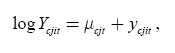
where μcjt is the mean log earnings in each cjt cell. Equation (4) is the first-stage estimation equation that extracts the individual earnings component from the earnings dynamics of the arrival cohort. A two-stage approach is standard in the literature on earnings inequality and earnings instability; however, in some studies ŷcjit are obtained by regressing log-earnings on an age polynomial (Haider 2001; Beach, Finnie and Gray 2003; Morissette and Ostrovsky 2005). The approach above appears more flexible in the context of this study.
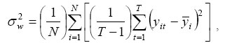
After obtaining ŷcjit from the first-stage regression, the variance of ŷcjit can be decomposed into 'between' and 'within' components. In the descriptive part of this study, it is simply assumed (as in Beach, Finnie and Gray 2003; Morissette and Ostrovsky 2005) that ycjit = ȳcji + vcjit, and both variance components are computed following the formulas in Johnston (1984).3
As different arrival cohorts are observed for a different number of years (for instance, the 1980- to-1982 cohort is observed for 22 years, while the 1998-to-2000 cohort is observed for only 4 years) it would be difficult to make a cross-cohort comparison of inequality and instability if calculations were made for all t's in which a cohort is observed. To make results comparable across cohorts, the decomposition is computed for a fixed number of post-arrival periods: t=4 (all cohorts), t=7 (all cohorts except that of 1998 to 2000) and t=10 (all cohorts except those of 1995 to 1997 and 1998 to 2000). For instance, if t=4 then the variance for the 1980-to-1982 arrival cohort is computed based on 1983, 1984, 1985 and 1986; the variance for the 1983-to-1985 arrival cohort is computed based on 1986, 1987, 1988 and 1989; and so on. The resulting panels are unbalanced because, for instance, in four-year panels, those who were present for only two or three periods are also included; similarly, seven-year panels include those who were observed for five or six periods and 10-year panels include those who were observed for eight or nine periods.
As mentioned in the introduction, the goal of this study is not only to document immigrant earnings inequality and earnings instability but also to analyse their potential causes, in particular, the role of pre-arrival education, language ability and country of birth. The effects of these variables can be estimated by adding control variables into the first-stage equation, re-estimating ycjit and using the new estimates of ycjit on the second stage. More specifically, Equation (4) takes the following form
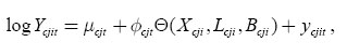
where Xcji is foreign education measured by the years of schooling, Lcji is a set of dummy variables reflecting the ability to speak either official language or both, and Bcji is the set of dummies related to the place of birth. A model that includes either Xcji, Lcji, Bcji, or the full set can be estimated. Hence, we can not only compare measures of earnings inequality and earnings instability across different arrival cohorts and arrival ages but also see the degree to which the earnings inequality and instability of each cohort are influenced by these variables. In the context of the Canadian immigrant selection process based on a point system4 that rewards foreign education and the ability to speak one of the official Canadian languages, such analysis may be particularly useful.
Although this is a very simple and intuitive method of analysing inequality and instability, it has obvious drawbacks. First, and most importantly, it does not allow for over-time changes in either permanent or transitory components. Second, it does not allow for the heterogeneity in earnings growth, as opposed to the heterogeneity in the levels of earnings. Finally, it ignores serial correlation in the transitory component. Hence, we will consider a more flexible model, similar to the models in Haider (2001) and Baker and Solon (2003).
We proceed as follows. Similar to (2), individual earnings of the members of cth arrival cohort who were j-years old at arrival are assumed to follow
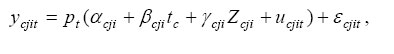
where ucjit = ucji,t−1 + rcjit and εcjit = ρεcji,t−1, + λt vcjit . Hence, total experience is broken down into two components: (1) 'Canadian experience,' tc, which is the same for all members of the cth arrival cohort, and (2) potential foreign experience Zcji, simply defined as the age at arrival minus 25.
From the residuals in (4), a sample auto-covariance matrix is constructed for each cohort and arrival age. For instance, for those who arrived during the 1980-to-1982 period at the age of 30, this will be a 22×22 matrix ( t=1983, 1984,…, 2004); for those who arrived during the 1995-to- 1997 period at the age of 30 this will be a 7×7 matrix ( t=1998, 1999,…, 2004). The size of the matrix will depend on both c and j; as the total number of arrival cohorts is seven, then for j ∈ [25,49] there will be 7×25=175 auto-covariance matrices Ωcj in total, which will produce 13,615 sample moments.
Let ωcj be a vector of unique elements of Ωcj,
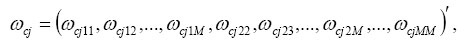
where M×M is the size of each Ωcj matrix depending on c and j. All ωcj can be stacked into a
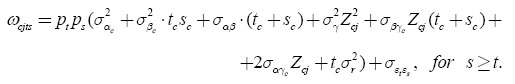
single vector Ω so that each diagonal element ωcjt in Ωcj can be written as

and each off-diagonal element ωcjts as
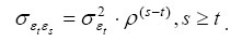
The transitory variance component εcjit = ρεcji,t−1 + λtνcjit takes the form of

and the covariance takes the form of
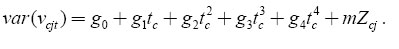
As in Baker and Solon (2003), σ2v can be modelled as a quadratic or quartic function of t and Zcj. In particular, it may be written as
Assuming that Ω* = f(t,s,Z;θ) is the population analog of Ω, we can now estimate the set of model parameters

by the generalized method of moments (GMM) using 13,615 sample moment corresponding to 13,615 elements in Ω
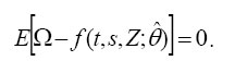
The parameters in (12) can be estimated using a GMM minimum distance estimator that chooses an optimal set of parameter estimates θ by minimizing
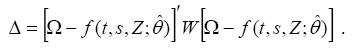
Haider (2001) and Baker and Solon (2003) point out the advantages of using an identity matrix as a weighting matrix in place of W (see also Altonji and Segal 1996, Clark 1996). One particular source of efficiency loss in an equal-weighted minimum distance estimator is that it ignores the fact that ωcj elements of Ω are based on a different number of observations. A more efficient estimator may be obtained if sample moments are weighted in proportion to the size of each cj cell. The estimation results in this study are based on a minimum-distance estimator that uses both an identity matrix as a weighting matrix and a weighting matrix that weights the sample moments according to their sample sizes.
It can be seen from (7) that setting p1983=1 (t=0) identifies σ2α in a model with a single σ2α parameter in the growth term. In a full model with cohort-specific parameters
 in the growth term, it is assumed
that
in the growth term, it is assumed
that 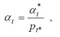 where t* is the first
loading factor for the cohort to which i belongs. For
instance, for the 1980-to-1982 cohort t*=1983; for the
1983-to-1985 cohort t*=1986; and so on. A diagonal element
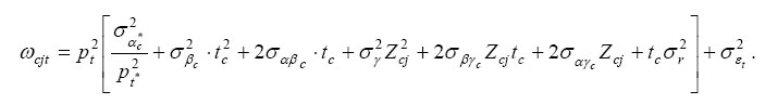
in Ωcjt can now be expressed as
where t* is the first
loading factor for the cohort to which i belongs. For
instance, for the 1980-to-1982 cohort t*=1983; for the
1983-to-1985 cohort t*=1986; and so on. A diagonal element
in Ωcjt can now be expressed as
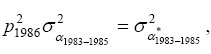
Hence, assuming Zcj=0, the permanent variance component for the 1980-to-1982 cohort in year 1983 (t=0) is
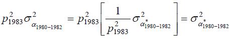 ; for the 1983-to-1985 cohort it is
 and so on. Put otherwise, all
 'absorb' the first loading factor for
the cohorts they represent. The estimates of
'absorb' the first loading factor for
the cohorts they represent. The estimates of  can be used instead of
  to construct cohort- specific
profiles of immigrant earning inequality.
to construct cohort- specific
profiles of immigrant earning inequality.
3 The within variance component is computed according to
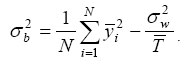
and the between variance component can be computed according to
4 The 'point system' introduced in Canada in 1967 rewards applicants with extra points for a higher education level, knowledge of official languages (English or French) and younger age.
- Date modified: