
Decomposition of gender wage inequalities through calibration: Application to the Swiss structure of earnings survey
Section 6. Application to the Swiss Structure of Earnings Survey
6.1 Data description
The dataset used contains information collected in 2008 by the Swiss Federal Statistical Office from a survey called Survey on Earnings Structure. A questionnaire was sent to public and private organizations from the secondary and tertiary sectors to collect information on particular aspects. These aspects include the size of the organization, employment contract types and employee remuneration within the organization. The questionnaire was filled in by an authorized member of the organization and not by employees. This enhances data reliability and makes it less prone to approximations. The analyses that follow were restricted to the private sector. The valid observations that were included were the individuals with no missing values, who worked more than one hour per week and whose difference between the age and the work experience was greater than or equal to 15 (according to the Swiss employment laws, this represents the legal minimum age to be eligible to work). Thus, 29,048 cases were excluded from the original dataset. The final dataset contains 647,139 men and 435,507 women. The sampling weights are also provided in the dataset by the Swiss Federal Statistical Office, therefore no treatment or computation of these weights were done in this application.
In the next tables, the values expressed in Swiss francs are given in parentheses. However, the figures are plotted using the logarithms of the wages. The values are obtained taking the survey weights into consideration.
Table 6.1 contains the median and wage averages for the entire sample and for women and men.
| Mean | Median | |
|---|---|---|
| Entire dataset | 6,977 | 5,905 |
| Women | 5,843 | 5,220 |
| Men | 7,725 | 6,346 |
Both the wage mean and the median values of men are above the values in the entire dataset, while those of women are below. Table 6.2 shows the distribution of women and men in low and high paying jobs. The weighted quantiles of the wage of the entire dataset are computed on the first row. The following two lines show the cumulative proportions of women and men who earn less than the value of the quantile.
| Quantile | |||||||||||
|---|---|---|---|---|---|---|---|---|---|---|---|
| 1% | 10% | 20% | 30% | 40% | 50% | 60% | 70% | 80% | 90% | 99% | |
| Logarithm of wage | 7.89 | 8.27 | 8.39 | 8.50 | 8.59 | 8.68 | 8.78 | 8.89 | 9.03 | 9.27 | 10.09 |
| (2,683) | (3,897) | (4,412) | (4,905) | (5,400) | (5,905) | (6,488) | (7,233) | (8,380) | (10,667) | (24,202) | |
| Cumulative proportion of women | 0.02 | 0.17 | 0.32 | 0.43 | 0.53 | 0.63 | 0.72 | 0.81 | 0.89 | 0.96 | 1 |
| Cumulative proportion of men | 0.006 | 0.06 | 0.12 | 0.21 | 0.31 | 0.42 | 0.52 | 0.63 | 0.74 | 0.86 | 0.99 |
While 43% of women have a wage of under CHF 4,905 (as opposed to only 21% of men), there are only 11% of women who earn between CHF 8,380 and CHF 24,202 (compared to 25% of men). Moreover, 63% of women earn below the median value of the wage of the entire dataset, compared to only 42% of men. The potential generating mechanisms of this allocation should be investigated. Nevertheless, it is not the purpose of this paper. For a closer insight into the distribution of the wages in each sample, Table 6.3 displays the weighted quantiles of the logarithms of the wages of women and men, as well as the difference between them. A surprising value of the difference between the wages is observed at the quantile of order 1%. It is expected that these jobs fall into the type of jobs that do not require extensive qualifications or high education levels. While only 0.6% of men occupy such positions (see Table 6.3), they earn more than the 2% of women who have similar jobs. Figure 6.1 shows the data presented in Table 6.3 below in a graphical form.
| Quantile | |||||||||||
|---|---|---|---|---|---|---|---|---|---|---|---|
| 1% | 10% | 20% | 30% | 40% | 50% | 60% | 70% | 80% | 90% | 99% | |
| Women | 7.80 | 8.19 | 8.30 | 8.38 | 8.47 | 8.56 | 8.66 | 8.76 | 8.88 | 9.06 | 9.67 |
| (2,432) | (3,602) | (4,005) | (4,344) | (4,756) | (5,220) | (5,743) | (6,353) | (7,154) | (8,577) | (15,761) | |
| Men | 8.01 | 8.36 | 8.49 | 8.58 | 8.67 | 8.76 | 8.86 | 8.98 | 9.14 | 9.38 | 10.26 |
| (3,000) | (4,259) | (4,850) | (5,344) | (5,820) | (6,346) | (7,012) | (7,908) | (9,291) | (11,905) | (28,571) | |
| Difference | 0.21 | 0.17 | 0.19 | 0.21 | 0.20 | 0.20 | 0.20 | 0.22 | 0.26 | 0.33 | 0.59 |
| (568) | (657) | (845) | (1,000) | (1,064) | (1,126) | (1,269) | (1,555) | (2,137) | (3,328) | (12,810) | |
The distance between the two sets of points increases toward the higher-level quantiles, which means that the differences between the wages become higher. It has to be established how much of these differences are not attributable to differing characteristics of women and men. As a final graphical evidence of wage inequalities, Figure 6.2 shows the distributions of the logarithm of the wages of women and men.
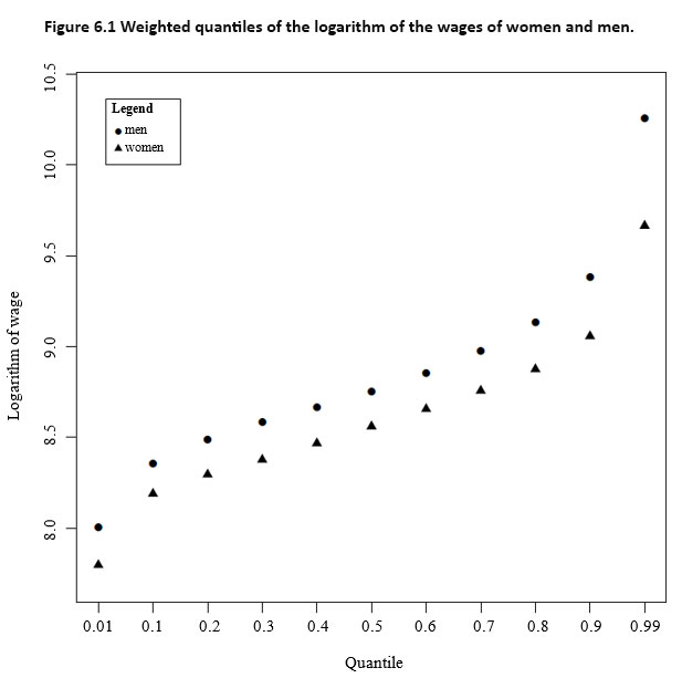
Description for Figure 6.1
Figure presenting the weighted quantiles of the logarithm of the wages of women and men. Quantiles are on the horizontal axis. The logarithm of the wages of women and men is on the vertical axis. The data are in the following table:
| Quantiles | Wage of women (Logarithm) | Wage of men (Logarithm) |
|---|---|---|
| 1% | 7.8 | 8.01 |
| 10% | 8.19 | 8.36 |
| 20% | 8.3 | 8.49 |
| 30% | 8.38 | 8.58 |
| 40% | 8.47 | 8.67 |
| 50% | 8.56 | 8.76 |
| 60% | 8.66 | 8.86 |
| 70% | 8.76 | 8.98 |
| 80% | 8.88 | 9.14 |
| 90% | 9.06 | 9.38 |
| 99% | 9.67 | 10.26 |
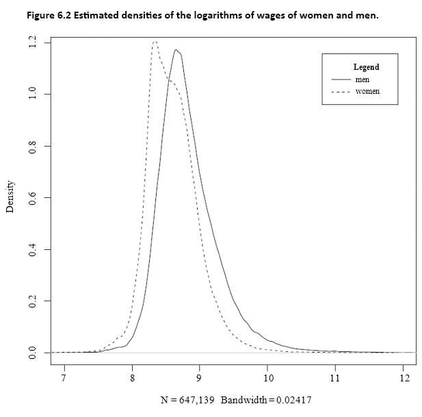
Description for Figure 6.2
Figure presenting the estimated density curves of the logarithms of wages of women and men. The density is on the y-axis, ranging from 0.0 to 1.2. The x-axis ranges from 7 to 12. Both densities overlap partially; the density associated to women wages reaches its highest point for a value of x smaller than then men one. The men wage curve is slightly shifted to the right.
6.2 The model
The regression model includes eight explanatory variables:
- education level : nominal variable with 9 categories indicating the highest educational degree attained;
- number of years of service in the current position (proxy for work experience);
- qualification requirements : ordinal variable with 4 levels indicating the level of qualification required for the position;
- region of the institution: nominal variable with 7 categories;
- economic sector: nominal variable with 10 categories;
- degree of occupation - the occupation rate of the employee (if the value is 1, then the employee works full-time);
- age: the actual age;
- the square of the age: the square of the age is also included, because it has been observed that the wage increases until a certain age and decreases afterwards (see, for instance Williams, 2010).
The model was selected from a number of models with several variables using the minimum AIC criterion. The dependent variable is the logarithm of the standardized wage. By standardized wage of an individual, we mean the wage computed for that individual if they worked full-time. This variable is provided by the Swiss Federal Statistical Office in the dataset, therefore no computation was done by the authors.
6.3 Weights and counterfactual distributions
This section only includes results in terms of logarithms. When using the BO method, the difference between average wages of men and women is 0.23, out of which only 0.09 represent the explained part and 0.14 the unexplained part. The results obtained through the methods presented above are compared. The calibration method through the chi-squared pseudo-distance is denoted as “linear”, the calibration through the Kullback-Leibler divergence as “raking-ratio” and the method proposed by DiNardo et al. (1996) adjusted to take the survey weights into consideration as “DFL”. First, Table 6.4 shows the minimum and the maximum values of the weights, as well as the standard deviations, obtained using the linear calibration, the raking-ratio calibration and the weighted DFL method.
| Method | Minimum | Maximum | Standard deviation |
|---|---|---|---|
| Linear | -39.06 | 319.8 | 4.97 |
| Raking-ratio | 0.0011 | 904.7 | 6.79 |
| Weighted DFL | 0.0022 | 804.4 | 6.16 |
The linear case yields the same results as the weighted BO method. However, as seen in Table 6.4, this particular case yields negative weights. There were 69,553 such weights (14.59%). The raking-ratio alternative always yields positive weights, however, the standard deviation of the weights is higher. The weighted DFL factor has a smaller standard deviation than the weights obtained by the raking-ratio calibration method. There are 1,319 cases where the conditional probability of being a man is larger than 0.98. Originally, the DFL factor is multiplied by the ratio between the sum of sampling weights of women and the sum of sampling weights of men. Since is smaller than one, the reweighting factor will shrink. If on the other hand, is larger than one (for instance, for sectors such as the public sector), the reweighting factor might be larger. Table 6.5 shows the structure effect estimated at the average levels of the wages. The two calibration approaches yield equal structure and composition effects. Using the DFL reweighting factor, results in a slightly lower structure effect and a higher composition effect than the other two methods.
| Method | Composition effect | Structure effect | Total |
|---|---|---|---|
| Linear | 0.09 | 0.14 | 0.23 |
| Raking-ratio | 0.09 | 0.14 | 0.23 |
| Weighted DFL | 0.10 | 0.13 | 0.23 |
Given that negative weights are obtained in the first case of calibration, the corresponding estimated density can not be graphically represented. Only women’s counterfactual wage distributions constructed using the raking-ratio and the DFL reweighting factor are constructed. They are presented in Figure 6.3.
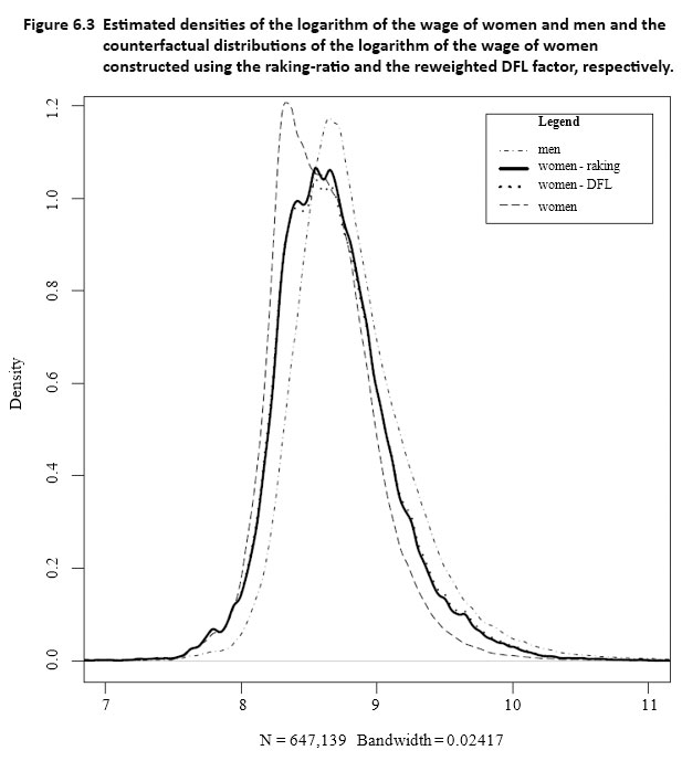
Description for Figure 6.3
Figure presenting four curves, namely the estimated densities of the logarithm of the wage of women and men and the counterfactual distributions of the logarithm of the wage of women constructed using the raking-ratio and the reweighted DFL factor. The density is on the y-axis, ranging from 0.0 to 1.2. The x-axis ranges from 7 to 12. The four curves overlap partially. Both counterfactual wage distributions are very close to each other around the tails, but differ toward the middle. Their highest points are less high and are located between those of the women and men wage densities.
Figure 6.3 shows that the two counterfactual wage distributions are very close to each other around the tails. However, toward the middle, the two methods do not yield the same results. As previously mentioned, using DFL reweighting and calibration methods allow the estimation the composition and structure effects not only at the average levels, but also along the entire distribution. Table 6.6 displays the estimated structure and composition effects of the wage differences between men and women computed using the three methods at some selected quantiles.
| Quantile | Method | Composition effect | Structure effect | Total |
|---|---|---|---|---|
| (%) | ||||
| 1% | Linear | 0.01 | 0.20 | 0.21 |
| (3%) | (97%) | |||
| Raking | -0.01 | 0.22 | 0.21 | |
| (-3.5%) | (103.5%) | |||
| Weighted DFL | -0.01 | 0.22 | 0.21 | |
| (-3.4%) | (103.4%) | |||
| 10% | Linear | 0.05 | 0.12 | 0.17 |
| (28.8%) | (71.2)% | |||
| Raking | 0.04 | 0.13 | 0.17 | |
| (22.4%) | (77.6%) | |||
| Weighted DFL | 0.03 | 0.14 | 0.17 | |
| (19.4%) | (80.6%) | |||
| 20% | Linear | 0.07 | 0.13 | 0.20 |
| (34.2%) | (65.8%) | |||
| Raking | 0.06 | 0.13 | 0.19 | |
| (29.7%) | (70.3%) | |||
| Weighted DFL | 0.05 | 0.14 | 0.19 | |
| (28.2%) | (71.8%) | |||
| 50% | Linear | 0.09 | 0.10 | 0.19 |
| (46.3%) | (53.7%) | |||
| Raking | 0.09 | 0.11 | 0.20 | |
| (44.7%) | (55.3%) | |||
| Weighted DFL | 0.09 | 0.11 | 0.20 | |
| (45.7%) | (54.3%) | |||
| 80% | Linear | 0.11 | 0.15 | 0.26 |
| (43.9%) | (56.1%) | |||
| Raking | 0.12 | 0.14 | 0.26 | |
| (46.5%) | (53.5%) | |||
| Weighted DFL | 0.13 | 0.13 | 0.26 | |
| (50.8%) | (49.2%) | |||
| 90% | Linear | 0.15 | 0.18 | 0.33 |
| (46.0%) | (54.0%) | |||
| Raking | 0.17 | 0.16 | 0.33 | |
| (51.6%) | (48.4%) | |||
| Weighted DFL | 0.19 | 0.14 | 0.33 | |
| (58.0%) | (42.0%) | |||
| 99% | Linear | 0.24 | 0.36 | 0.60 |
| (40.0%) | (60.0%) | |||
| Raking | 0.27 | 0.33 | 0.60 | |
| (45.3%) | (54.7%) | |||
| Weighted DFL | 0.29 | 0.30 | 0.59 | |
| (49.4%) | (50.6%) | |||
The proportion of the structure effect of the entire wage difference between men and women decreases as the order of the quantile increases. This means that for jobs with higher salaries, more of the wage differences can be explained by differences in group characteristics than for jobs with lower salaries. The raking-ratio and the DFL reweighting factor yield similar results up to the quantile of order 90%. The composition effect at the first percentile is estimated to be negative, meaning that at this point, the differences in wages are due solely to discrimination.
Figure 6.4 shows the weighted quantiles of the logarithms of the wage of men, those of women and contrast the counterfactual distributions obtained through the raking-ratio calibration and the DFL reweighting factor. Because the linear calibration yielded negative weights, the same graph is not reproduced for it.
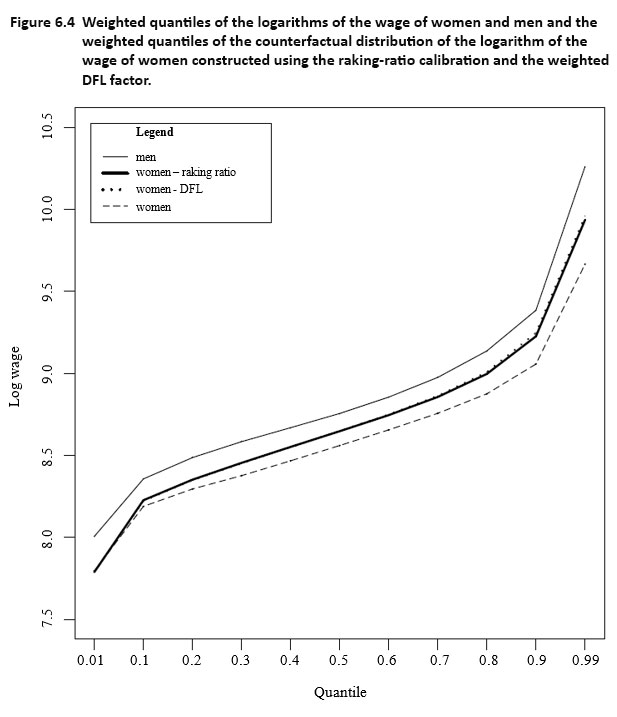
Description for Figure 6.4
Figure showing four curves, namely the weighted quantiles of the logarithms of the wage of women and men and those of the counterfactual distribution of the logarithm of the wage of women constructed using the rakingratio calibration and the weighted DFL factor. The wage logarithm is on the y-axis, ranging from 7.5 to 10.5. The quantiles are on the x-axis, ranging from 0.01 to 0.99. The curve associated to the men wages is higher than the other three. The three curves associated to the women wages have the same starting point, but from quantile 0.1, the logarithms of the wage of women is lower than those of the two counterfactual distributions. The raking-ratio and the DFL reweighting factor yield similar results up to the quantile of order 90% where the latter starts to be slightly higher.
6.4 Further decomposition of the structure effect
A logistic model for the probability of being a man yields estimated values between 0.002 and 0.99. For the variables “years in the current position”, “age” and “square of the age” the difference between the average values of men and the reweighted averages of women computed using the reweighting factor are the largest. In equation (4.8), the structure effect is composed of the pure effect and the residual effect. Using the DFL reweighting factor, the residual effect equals -0.00474. In contrast, by using either one of the calibration techniques, in both cases, it equals 0. Moreover, the calibration approach allows overriding the computation of the counterfactual regression coefficients. This is because the technique ensures the equality between the means and Calibration thus represents a generalization of the DFL reweighting factor technique, because it allows for a more precise estimation of the structure effect, since the resulting value only includes the pure part.
- Date modified: