
The anchoring method: Estimation of interviewer effects in the absence of interpenetrated sample assignment
Section 6. Discussion
We have developed and evaluated a new method for estimating interviewer effects in the absence of interpenetrated assignment of sampled units to interviewers. Via a simulation study and applications using real survey data from the BRFSS, we have demonstrated the ability of the proposed anchoring method to improve estimates of interviewer effects in situations where interpenetrated assignment may not be feasible and interviewer variance may be arising from the underlying sample assignments. The anchoring method can also easily be applied in a Bayesian framework, leveraging prior information to improve the quality of predictions and inferences related to interviewer components of variance.
In interviewer-administered survey data collections, interviewer effects should generally be monitored as part of an ongoing data collection to prevent excessive problems with interviewer variance in survey outcomes at the conclusion of the data collection. Survey managers responsible for this type of monitoring will likely benefit from the anchoring method, improving any real-time intervention decisions made for individual interviewers in a responsive survey design framework. Real-time interventions/re-trainings for interviewers who are found to have extreme effects on production outcomes or variables of scientific interest that in reality only reflect the features of the areas in which they are working and not actual interviewer performance will be at best inefficient and at worst could cause interviewers who are otherwise performing well to be inappropriately criticized and perhaps to leave a given study.
When using the anchoring method in practice, we would suggest that it be described as a method that “adjusts estimates of interviewer variance components for spurious within-interviewer correlation in survey measures of interest that can arise due to non-random assignment of sampled units to interviewers.” We emphasize the importance of a sound theoretical selection of an anchoring variable (or variables) that ideally has the optimal properties described in this paper. In the absence of an anchoring variable with these optimal properties, we argue that “clean” estimation of interviewer variance in a non-interpenetrated sample design may simply not be possible, and that analysts 1) adjust for as many respondent-, interviewer-, and area-level covariates as possible when attempting to estimate the interviewer variance, and 2) report estimates of uncertainty associated with the estimated variance components, preferably using Bayesian approaches. This will prevent over-estimation of interviewer variance components and possible attribution of lower data quality to interviewers that are already performing extremely challenging tasks in the field.
There are several limitations to our proposed method. Perhaps the largest is the requirement for “anchoring” variables to not be subject to interviewer error and still be highly correlated with the substantive variable of interest. In our BRFSS example, we considered age, gender, race, and education as “anchoring” self-rated health. Although age is self-reported and thus possibly subject to some degree of measurement error (for example, reporting younger ages or rounding ages), we do not see an obvious mechanism by which this would be induced by the interviewer, although of course that possibility remains. A similar argument can be made for the other three factors, although the possibility of interviewer induced measurement error is slightly stronger due to issues such as “liking” between interviewers and respondents (West and Blom, 2017). In addition, the normality assumption that we make in the paper is highly restrictive. To deal with this in our application, we replaced the multivariate anchoring model (3.2) with a model that summarized the multiple anchors into a linear predictor that we then used in the bivariate anchoring model (3.1). While this linear predictor is effectively a sufficient statistic in the case where all of the anchoring variables are normal, as shown in the simulation study, it is more of an ad-hoc solution when some or all of the anchoring variables are non-normal, as was the setting in our application.
A more principled solution when one or more of the components of are dichotomous variable would be to consider extensions such as probit random effects models, replacing in (3.1) with a latent where the observed and the variance for identifiability, for all values of where is dichotomous. More ambitiously, we could use a Gaussian random effects copula model (Wu and de Leon, 2014) for arbitrary distributions for Standard software will not accommodate such models, although methods that integrate over random effects or use fully Bayesian approaches could be considered. Next, while other sources of measurement error are potentially important to address in inference, our focus here is on measurement error variance introduced by interviewer effects and its estimation in the absence of interpenetration. Finally, we note that our approach, like its competitors, relies on observed data and is thus not a replacement for true interpenetration, which ensures that all forms of non-random assignment (observed and unobserved) are eliminated.
In addition to extending the anchoring method to the case of regression coefficients and non-normal variables, future applications also need to consider contexts where the correlations of the anchoring variables with the survey variables of interest that may be prone to interviewer effects are modest at best. Our simulation study suggests that good anchoring variables having strong associations with the survey variables of interest are important for the effectiveness of this method, and future studies should also focus on the identification of sound anchoring variables (like age, education, etc.) that are unlikely to be affected by interviewers and could serve as useful anchors in other applications.
Acknowledgements
Funding for this research was provided by NIH Grant #1R01AG058599-01. The authors would like to thank the editor, associate editor, and two reviewers for their guidance which has improved the manuscript.
Supplemental materials
SAS code implementing the different approaches
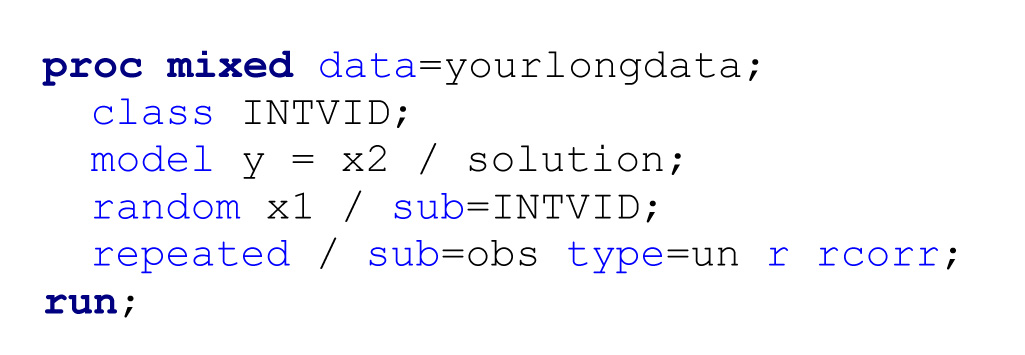
The SAS code below can be used to implement the anchoring method using a standard frequentist approach. Implementing this approach requires the data to be in a “long” structure with two observations per subject (corresponding to the two variables), where the variable X2 is an indicator variable for the anchoring variable (1 = the observation on Y is the anchor, 0 = the observation on Y is the variable of interest), the variable X1 is an indicator for the variable of interest (1 = the observation on Y is the variable of interest, 0 = the observation on Y is the anchor), INTVID is the interviewer ID, and OBS is a subject ID:
Description of SAS code 6.1
proc mixed data=yourlongdata;
class INTVID;
model y = x2 / solution;
random x1 / sub=INTVID;
repeated / sub=obs type=un r rcorr;
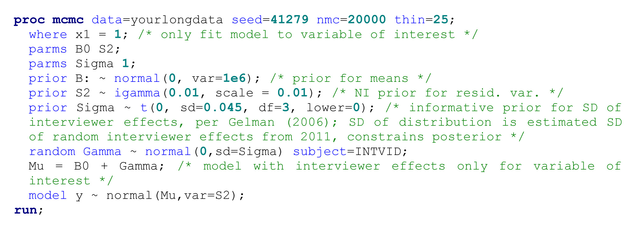
run; The SAS code below can be used to fit the naïve model using a Bayesian approach with a weakly informative prior. This approach requires the data to be in the same “long” format:
Description of SAS code 6.2
proc mcmc data=yourlongdata seed=41279 nmc=20000 thin=25;
where x1 = 1; /* only fit model to variable of interest */
parms B0 S2;
parms Sigma 1;
prior B: ~ normal(0, var=1e6); /* prior for means */
prior S2 ~ igamma(0.01, scale = 0.01); /* NI prior for resid. var. */
prior Sigma ~ t(0, sd=0.045, df=3, lower=0); /* informative prior for SD of interviewer effects, per Gelman (2006);
SD of distribution is estimated SD of random interviewer effects from 2011, constrains posterior */
random Gamma ~ normal(0,sd=Sigma) subject=INTVID;
Mu = B0 + Gamma; /* model with interviewer effects only for variable of interest */
model y ~ normal(Mu,var=S2);
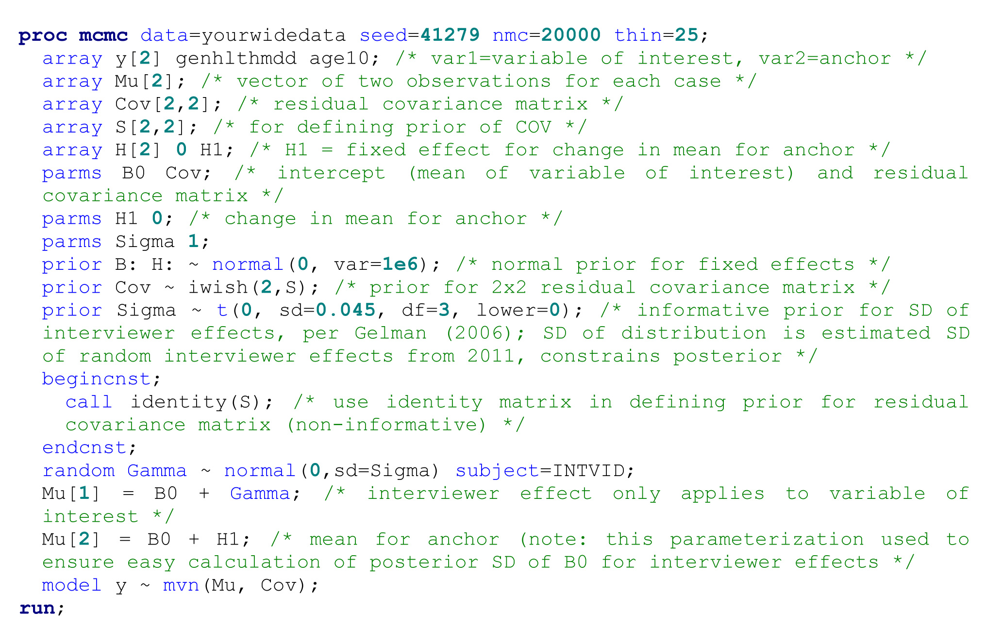
run; Finally, the SAS code below can be used to implement the anchoring method using a Bayesian approach with a weakly informative prior. Implementing this approach requires the data to be in a wide structure, with one row per case and interviewer IDs (INTVID):
Description of SAS code 6.3
proc mcmc data=yourwidedata seed=41279 nmc=20000 thin=25;
  array y[2] genhlthmdd age10; /* var1=variable of interest, var2=anchor */
  array Mu[2]; /* vector of two observations for each case */
  array Cov[2,2]; /* residual covariance matrix */
  array S[2,2]; /* for defining prior of COV */
  array H[2] 0 H1; /* H1 = fixed effect for  change in mean for anchor */
  parms B0 Cov; /* intercept (mean of variable of interest) and residual covariance matrix */
  parms H1 0; /* change in mean for anchor */
  parms Sigma 1;
  prior B: H: ~ normal(0, var=1e6); /* normal prior for fixed effects */
  prior Cov ~ iwish(2,S); /* prior for 2x2 residual  covariance matrix */
  prior Sigma ~ t(0, sd=0.045, df=3, lower=0); /* informative prior for SD of interviewer effects, per Gelman (2006);
  SD of distribution is estimated SD of random interviewer effects from 2011, constrains posterior */
  begincnst;
  	call identity(S); /* use identity matrix in defining prior for residual covariance matrix (non-informative) */
  endcnst;
  random Gamma ~ normal(0,sd=Sigma) subject=INTVID;
  Mu[1] = B0 + Gamma; /* interviewer effect only applies to variable of  interest */
  Mu[2] = B0 + H1; /* mean for anchor (note:  this parameterization used to ensure easy calculation
  of posterior SD of B0 for interviewer effects */
  model y ~ mvn(Mu, Cov);
run;
References
Biemer, P.P. (2010). Total survey error: Design, implementation, and evaluation. Public Opinion Quarterly, 74(5), 817-848.
Biemer, P.P., and Stokes, S.L. (1985). Optimal design of interviewer variance experiments in complex surveys. Journal of the American Statistical Association, 80(389), 158-166.
Brunton-Smith, I., Sturgis, P. and Williams, J. (2012). Is success in obtaining contact and cooperation correlated with the magnitude of the interviewer variance? Public Opinion Quarterly, 76, 265-286.
Carle, A.C. (2009). Fitting multilevel models in complex survey data with design weights: Recommendations. BMC Medical Research Methodology, 9, 49-62.
Centers for Disease Control (2013). Behavioral Risk Factor Surveillance System: OVERVIEW: BRFSS 2012. Accessed at http://www.cdc.gov/brfss/annual_data/2012/pdf/Overview_2012.pdf.
Cernat, A., and Sakshaug, J.W. (2021). Interviewer effects in biosocial survey measurements. Field Methods, 33, 236-252.
Durrant, G.B., Groves, R.M., Staetsky, L. and Steele, F. (2010). Effects of interviewer attitudes and behaviors on refusal in household surveys. Public Opinion Quarterly, 74, 1-36.
Elliott, M.R., and West, B.T. (2015). “Clustering by interviewer”: A source of variance that is unaccounted for in single-stage health surveys. American Journal of Epidemiology, 182, 118-126.
Fellegi, I.P. (1974). An improved method of estimating the correlated response variance. Journal of the American Statistical Association, 69,496-501.
Fowler, F.J., and Mangione, T.W. (1989). Standardized Survey Interviewing: Minimizing Interviewer-Related Error. Newbury Park: Sage.
Franks, P., Gold, M.R. and Fiscella, K. (2003). Sociodemographics, self-rated health, and mortality in the US. Social Science & Medicine, 56, 2505-2514.
Gao, S., and Smith, T.M.F. (1998). A constrained MINQU estimator of correlated response variance from unbalanced data in complex surveys. Statistica Sinica, 8, 1175-1188.
Gelman, A. (2006). Prior distributions for variance parameters in hierarchical models. Bayesian Analysis, 1, 515-533.
Groves, R.M. (2004). Chapter 8: The interviewer as a source of survey measurement error. Survey Errors and Survey Costs (2nd Edition). New York: Wiley-Interscience.
Groves, R.M., and Magilavy, L.J. (1986). Measuring and explaining interviewer effects in centralized telephone surveys. Public Opinion Quarterly, 50, 251-266.
Heeringa, S.G., West, B.T. and Berglund, P.A. (2017). Applied Survey Data Analysis, Second Edition. Boca Raton, FL: Chapman Hall/CRC Press.
Hox, J.J. (1994). Hierarchical regression models for interviewer and respondent effects. Sociological Methods and Research, 22, 300-318.
Joffe, M.M., Ten Have, T.R., Feldman, H.I. and Kimmel, S.E. (2004). Model selection, confounder control, and marginal structural models: Review and new applications. The American Statistician, 58, 272-279.
Kalton, G. (1983). Introduction to Survey Sampling, Sage Publications: London, UK.
Kish, L. (1962). Studies of interviewer variance for attitudinal variables. Journal of the American Statistical Association, 57, 92-115.
Kish, L. (1965). Survey Sampling. New York: John Wiley & Sons, Inc.
Kleffe, J., Prasad, N.G.N. and Rao, J.N.K. (1991). “Optimal” estimation of correlated response variance under additive models. Journal of the American Statistical Association, 86, 144-150.
Laird, N.M., and Ware, J.H. (1982). Random-effects models for longitudinal data. Biometrics, 38, 963-974.
Lepkowski, J.M., Mosher, W.D., Groves, R.M., West, B.T., Wagner, J. and Gu, H. (2013). Responsive design, weighting, and variance estimation in the 2006-2010 National Survey of Family Growth. National Center for Health Statistics. Vital Health Stat, 2(158).
Liang, K.-Y., and Zeger, S.L. (1986). Longitudinal data analysis using generalized linear models. Biometrika, 73, 13-22.
O’Muircheartaigh, C.A., and Campanelli, P. (1998). The relative impact of interviewer effects and sample design effects on survey precision. Journal of the Royal Statistical Society, Series A, 161, 63-77.
Pfeffermann, D., Skinner, C.J., Holmes, D.J., Goldstein, H. and Rasbash, J. (1998). Weighting for unequal selection probabilities in multilevel models. Journal of the Royal Statistical Society, Series B, 60, 23-40.
Rabe-Hesketh, S., and Skrondal, A. (2006). Multilevel modelling of complex survey data. Journal of the Royal Statistical Society-A, 169, 805-827.
Rasbash, J., and Goldstein, H. (1994). Efficient analysis of mixed hierarchical and cross-classified random structures using a multilevel model. Journal of Educational and Behavioral Statistics, 19, 337-350.
Rohm, T., Carstensen, C.H., Fischer, L. and Gnambs, T. (2021). Disentangling interviewer and area effects in large-scale educational assessments using cross-classified multilevel item response models. Journal of Survey Statistics and Methodology, 9, 722-744.
Sakshaug, J.W., Tutz, V. and Kreuter, F. (2013). Placement, wording, and interviews: identifying correlates of consent to link survey and administrative data. Survey Research Methods, 7, 133-144.
Schaeffer, N.C., Dykema, J. and Maynard, D.W. (2010). Interviewers and Interviewing. In Handbook of Survey Research, Second Edition (Eds., J.D. Wright and P.V. Marsden), Bingley, U.K.: Emerald Group Publishing Limited.
Schnell, R., and Kreuter, F. (2005). Separating interviewer and sampling-point effects. Journal of Official Statistics, 21, 389-410.
Skinner, C.J., Holt, D. and Smith, T.M.F. (1989). Analysis of Complex Surveys. New York: John Wiley & Sons, Inc.
Stiratelli, R., Laird, N. and Ware, J. (1984). Random effects models for serial observations with binary responses. Biometrics, 40, 961-971.
Vassallo, R., Durrant, G. and Smith, P. (2017). Separating interviewer and area effects by using a cross-classified multilevel logistic model: Simulation findings and implications for survey designs. Journal of the Royal Statistical Society, Series A, 180, 531-550.
Veiga, A., Smith, P.W.F. and Brown, J.J. (2014). The use of sample weights in multivariate multilevel models with an application to income data collected by using a rotating panel survey. Journal of the Royal Statistical Society (Series C), 63, 65-84.
von Sanden, N., and Steel, D. (2008). Optimal estimation of interviewer effects for binary response variables through partial interpenetration. Centre for Statistical and Survey Methodology, University of Wollongong, Working Paper 04-08.
West, B.T., and Blom, A.G. (2017). Explaining interviewer effects: A research synthesis. Journal of Survey Statistics and Methodology, 5, 175-211.
West, B.T., and Elliott, M.R. (2014). Frequentist and Bayesian approaches for comparing interviewer variance components in two groups of survey interviewers. Survey Methodology, 40, 2, 163-188. Paper available at https://www150.statcan.gc.ca/n1/en/pub/12-001-x/2014002/article/14092-eng.pdf.
West, B.T., and Olson, K. (2010). How much of interviewer variance is really nonresponse error variance? Public Opinion Quarterly, 74, 1004-1026.
West, B.T., Kreuter, F. and Jaenichen, U. (2013). “Interviewer” effects in face-to-face surveys: A function of sampling, measurement error or nonresponse? Journal of Official Statistics, 29, 277-297.
Wu, B., and de Leon, A.R. (2014). Gaussian copula mixed models for clustered mixed outcomes, with application in developmental toxicology. Journal of Agricultural, Biological, and Environmental Statistics, 19, 39-56.
- Date modified: