
Developments in machine learning series: Issue three
By: Nicholas Denis, Statistics Canada
This month's topics:
- Advanced generative modelling now available for tabular data
- Filling in the blanks is all you need
- Masked autoencoders for tabular data imputation
Advanced generative modelling now available for tabular data
Denoising diffusion probabilistic models can be applied to any tabular dataset and handle any feature type to generate synthetic data that can sometimes be more effective than real data.
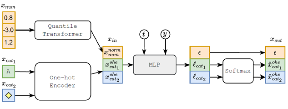
Figure 1: TabDDPM scheme for classification problem; t, y, and l denote a diffusion timestep, a class label, and logits, respectively.
Data passing through TabDDPM. A tabular data instance, , is composed of numerical (num) and categorical (cat) features. Numerical features are transformed using the quantile transformer, and categorical features are one-hot encoded. The forward noise process is computed and corrupts the transformed input at timestep, , which is used as input into TabDDPM. TabDDPM is a multi-layer perceptron (MLP) and conditioned on the diffusion timestep, , and class label, . The output of TabDDPM is the estimated noise added to the numerical features, , and the estimated uncorrupted (original) one-hot encoded categorical features.
The flowchart has the following elements:
- Quantile Transformer (: 0.8, -3.0, 1.2)
- Forward to 3.
- One-hot Encoder (, )
- Forward to 3.
- X in (, ),
- Forward to 4.
- MLP
- t forward to 4.
- Y forward to 4.
- Forward to 5.
- , ,
- forward to 7.
- , forward to 6.
- Softmax
- From forward to 7.
- From forward to 7.
- X out (, , )
What's new? Denoising diffusion probabilistic models (DDPM) produce incredible results in text-to-image generation (e.g. Imagen, Stable Diffusion, DALL-E 2) and have been applied to tabular datasets. This has enabled synthetic tabular data instances to be generated comprising both numerical and categorical features.
How it works: A typical DDPM uses a forward Gaussian noising process and a reverse (learned) denoising process to transform pure noise sampled from a standard multivariate normal distribution to a synthetic data instance. Similarly, tabular data with diffusion models (TabDDPM) also includes a multinomial diffusion process that allows DDPM to be applied to categorical, ordinal and Boolean features typically found in tabular data.
Why does it work? For a quick review of DDPM models and the Gaussian diffusion process, please see Developments in Machine Learning Series: Issue two. Here, we'll focus on the multinomial diffusion process:
- Let be a one-hot encoded variable of K dimensions (categories).
- A forward diffusion process, , over T time steps is written as:
Where , is a noise schedule.
- The posterior, is well defined, and the reverse diffusion process is approximated using a neural network: The network can maximize the variational lower bound (KL divergences within the reverse diffusion process).
- Numerical features are transformed using the quantile transformer, and categorical (ordinal, Boolean, etc) features are transformed to one-hot encodings. Gaussian and multinomial diffusion models are trained on each feature type, respectively.
Results: Several baseline generative models are compared, including generative adversarial networks (GAN) and a variational autoencoder (VAE), specifically designed for tabular datasets. There are 15 tabular datasets that are used. The authors use a formalized and standardized approach to evaluate the quality of the synthetic data generated by a generative model, called ML Efficiency. The approach is worth explaining in detail for anyone interested in evaluating the quality of synthetic datasets.
First, the real data is fit to a CatBoost classifier using a fixed hyperparameter tuning budget and a hyperparameter optimization tool called Optuna. Once the optimal hyperparameters are found, a CatBoost model is trained using the synthetic data. The F1 score of the model, evaluated on real data is called the ML Efficiency score. This metric measures the quality of synthetic data by its ability to be used instead of real data for downstream ML tasks.
- TabDDPM beat the other deep learning approaches in 14/15 datasets
- On 5/15 datasets, a CatBoost model trained on synthetic data from TabDDPM achieved higher test accuracy than a CatBoost model trained on real data.
Why does it matter? DDPMs are producing realistic synthetic data in other modalities. Sampling high-quality synthetic tabular data instances can have applications in data augmentation – generating and sharing synthetic versions of sensitive datasets that can guarantee privacy, imputation and balance class imbalanced datasets.
But… When tested, synthetic minority oversampling technique (SMOTE) consistently outperformed TabDDPM, despite being an older, simpler technique that generates novel data instances by taking convex combinations of data instances from within the dataset. Moreover, TabDDPM is computationally expensive to train, especially with their Optuna hyperparameter optimization approach.
Our opinion: With access to a GPU (graphics processing unit) for model training, TabDDPM is a great way to generate high-quality synthetic tabular data and will remain a strong baseline for future improvements in tabular DDPMs.
Filling in the blanks is all you need
Researchers from Facebook AI Research have achieved state-of-the-art performance on the ImageNet-1K dataset by applying the same pre-training task to computer vision datasets, as was applied to the successful language models.
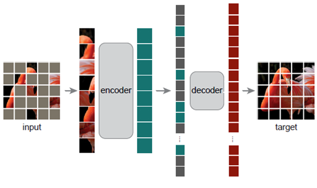
Figure 2: Masked autoencoder architecture. 75% of the pixel patches are masked and then reconstructed as a pretraining task.
An image of masked autoencoder architecture.
Input image of a pixelated flamingo, with most of the pixels greyed out. Forward to encoder containing all the unmasked pixels. Forward to decoder, containing only masked pixels. Forward to the final target – an image of the pixelated flamingo, no masked pixels.
What's new? Masked autoencoders (MAE) combine the Vision Transfer (ViT) architecture and the masked token prediction pre-training task from BERT (Bidirectional Encoder Representations from Transformers)-style language models to produce state-of-the-art performance on various computer vision tasks and datasets.
How does it work? BERT-style language models encode and represent natural language via a Masked Language Model pre-training task. When given a large amount of text data, a sentence is fed into the model with 15% of the input word tokens masked. By correctly inferring the masked words, BERT-style models capture the semantics of the text inputs, making them useable for downstream natural language processing tasks, like text classification. MAE uses the same approach, except instead of masking words, 75% of the image's pixel patches are masked and reconstructed.
Why does it work? MAE uses an asymmetric encoder and decoder architecture. Both the encoder and decoder are transformer models. Since 75% of the image patches are masked, only 25% are processed by the encoder, making it more computationally efficient than traditional ViTs for standard supervised learning. The decoder also has a smaller architecture and reconstructs the masked patches. By minimizing the reconstruction loss, the model learns to extract global information about an image, including the masked patches, solely from the ‘visible' patch pixels. After pre-training is complete, the decoder is discarded, and the encoder acts as a pre-trained model which can be used as-is to transform inputs for linear classification or can be fine-tuned.
Results:
- Using the ImageNet-1K (IN1K) dataset, MAE pre-training and then fine-tuning for 50 epochs achieved higher accuracy than the previous state-of-the-art fully supervised model.
- Using various standard ViT architectures, MAE consistently outperformed previous state-of-the-art self-supervised pre-training techniques on the IN1K dataset for classification, on the COCO dataset for object detection and instance segmentation, and on the ADE20k dataset for semantic segmentation.
- When evaluated for transfer learning, MAE outperformed all previous state-of-the-art accuracy results for various iNaturalist and Places datasets; even by as much as 8%.
Our opinion: Pre-training techniques are becoming increasingly powerful and can now outperform standard supervised learning paradigms. MAE is not only impressive in its results but is also impressively simple. This paper doesn't use any bells, whistles, or any special tricks. Moreover, they use the basic ViT architecture, and expect significant result improvements by using advanced vision transformer architectures.
Though relatively new, MAE has been applied to spatiotemporal data, Multi-modal data, tabular data, and is here to stay with applications beyond pre-training for supervised learning. It's been used for data imputation and can be used for semi-supervised learning. Pre-trained MAE models can also be downloaded and used by visiting Github Facebookreseearch/mae.
Masked autoencoders for tabular data imputation
Researchers turn an imputer into an imputer. Wait, is that right?
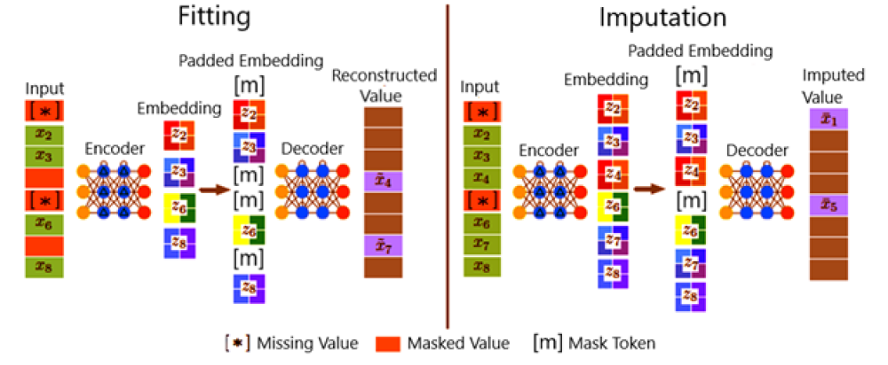
Figure 3: Overall, framework of ReMasker.
During the fitting stage, for each input, in addition to its missing values, another subset of values (re-masked values), is randomly selected and masked out. The encoder is applied to the remaining values to generate its embedding, which is padded with mask tokens and processed by the decoder to re-construct the re-masked values. During the imputation staged, the optimized model is applied to predict the missing values.
Fitting stage:
Input, encoder, embedding, forward to padded embedding, decoder and reconstructed value.
Imputation stage:
Input, encoder, embedding forward to padded embedding, decoder and imputed value.
What's new? As described above, MAEs are trained to impute missing data. Researchers decided to do the unthinkable and apply MAE to tabular data in order to… impute missing data.
How does it work? MAE and the masked token prediction task were originally developed to pre-train an encoder that could be fine-tuned for downstream classification. In the original MAE implementation, the decoder was discarded after pre-training. In ReMasker, the encoder and decoder are kept, and then applied to actual missing values in the dataset to infer their values.
Why does it work? ReMasker is trained with a tabular dataset that has actual missing values. During training, each input is masked via a masking mechanism and produces an input with a mixture of visible values, masked values, and missing values. The visible values enter the encoder (transformer architecture), and the output tokens are combined with learnable mask tokens and positional encodings for the masked and missing features. These then pass through the decoder (transformer architecture). The model then infers the original value of the masked features, but not the actual missing values.
At test time no additional masking is used, and the data instances with missing features are applied to ReMasker to infer the missing values. Just as the authors of the original MAE paper suggest, the encoder learns to represent the global information of an image from the visible pixel patches, the authors of ReMasker claim that the encoder learns a "missingness-invariant" representation of the data. In doing so, ReMasker learns to represent tabular data instances in a discriminative manner that is robust to missing features.
Results: The authors perform experiments using 12 tabular datasets from the UCI Machine Learning Repository, consider three different mechanisms to sample missing values, and compare ReMasker to 13 state-of-the-art imputation techniques. Performance metrics included Root Mean-Squared Error of imputed vs. real values, Wasserstein Distance of imputed vs. real data, and Area Under the Receiving Operating Characteristic (AUROC) curve, measuring effectiveness of imputed data for downstream classification tasks.
- ReMasker consistently matched or outperformed almost all the baseline imputing approaches, most or all of the time.
- The closest imputing approach was HyperImpute, a new and state-of-the-art imputation approach that uses an ensemble of imputation methods and selects the best imputation model for each column of a dataset.
- Empirical evidence suggested that ReMasker performance increases as the dataset size increases, as well when the number of features increases.
- ReMasker is robust to the amount of missing values, performing consistently from 10% to 70% of features missing.
- Since HyperImpute is an Ensembling approach, the authors included ReMasker as a possible base model within HyperImpute and showed that it further improved the results of HyperImpute.
- To test their hypothesis that by applying MAE pre-training on tabular data, it allows the encoder to learn "missing-ness invariant" representations of the data, the authors computed the Centered Kernel Alignment between the encodings of the full data and the encodings of the data with missing values between 10% and 70%. They found the similarity was robust and only slightly decreased as the proportion of missing features increased, providing evidence in support of their hypothesis.
What's the context? Real world datasets contain missing data for many reasons. The use of data for ML models, official statistics, or inference of any kind must address how to or how not to use data with missing values. Imputation is important and an active area of research within ML and statistical methods communities.
Our opinion: Given that the MAE pre-training technique explicitly performs imputation, it was only a matter of time before a researcher tested its applicability for imputation on tabular datasets. This was a good first look into how MAE could be used for such purposes.
Meet the Data Scientist

If you have any questions about my article or would like to discuss this further, I invite you to Meet the Data Scientist, an event where authors meet the readers, present their topic and discuss their findings.
Thursday, March 16
2:00 to 3:30 p.m. ET
MS Teams – link will be provided to the registrants by email
Register for the Data Science Network's Meet the Data Scientist Presentation. We hope to see you there!
Subscribe to the Data Science Network for the Federal Public Service newsletter to keep up with the latest data science news.
- Date modified: