
By Stany Nzobonimpa, Mohamed Abou Hamed, Ilia Korotkine, Tiffany Gao, Housing, Infrastructure and Communities Canada
Acknowledgements
The authors would like to acknowledge the following individuals for their contributions and support of the project: Kate Burnett-Isaacs, Director of Data Science and Matt Steeves, Senior Director of Engineering, Technical and Project Operations - Major Bridges and Projects.
Introduction
The identification and flagging of events such as data points that significantly deviate from standard or expected behaviour is known as anomaly detection in the field of data science. Anomalies are of special interest to data scientists because their presence signals underlying issues that prompt suspicions and usually warrants investigations. Various statistical techniques have historically been applied to answer anomaly-related questions and advances in Artificial Intelligence (AI) have made the exercise one of the most known applications of ML frameworks and approaches.
In this article, we present and discuss key findings of a project applying anomaly detection to sensor data. The project was carried out at HICC by a multi-disciplinary team of data scientists and engineers. While the project is multi-phased, this article reports on methods and results of the first phase in which sensor data from a federal bridge was used for early detection of anomalous readings.
The article is structured as follows: we start by a short review of relevant and recent literature on anomaly detection and its applications where we show that methods for data anomaly detection have evolved and continue to do so. After reviewing the literature, we present the problem, the methods, and results of this first phase of the project. In particular, we show that the approach enabled us to proactively, in a timelier and less laborious manner, flag anomalies in the generated sensor data that could have otherwise been missed. Indeed, our results show that for the period of April 2020 to September 2024, a number of sensor readings were successfully flagged as anomalies using the methods that we present in this paper. We conclude by stating the next steps of the project.
Literature Review
The application of machine learning to anomaly detection
Anomaly detection has long been a focus in data mining, which laid the groundwork for many modern ML approaches. Foundational works in data mining have explored anomaly detection techniques extensively, including clustering-based, distance-based, and density-based methods. Thus, anomaly detection is one of the core applications of ML technology that has been applied by AI practitioners for decades (Nassif et al., 2021). In its simplest form, anomaly detection is known as outlier detection and consists of flagging data points that significantly deviate from or do not conform with the majority of data. The multiple applications of anomaly detection from fields as diverse as medical research, cybersecurity, financial fraud, and law enforcement have attracted both researchers and practitioners’ interests and resulted in a flourishing literature on the topic (Chandola et al. 2009).
Traditionally, anomaly detection could be completed manually by examining and filtering data and using context knowledge to provide insights on the detected behaviours. As datasets get larger, statistical approaches have been useful in detecting anomalies. For example, Soule et al., (2005) proposed a combination of filtering using Kalman filters and other statistical techniques to detect volume anomalies in large networks. The authors argue that anomaly detection can always be viewed as a problem of statistical hypothesis testing and they use behaviours, residual means, and variance changes over time to compare four different statistical approaches to anomaly detection (pp.333-338).
Using receiver operating characteristic (ROC) curves for binary normal vs anomaly illustrations, Soule et al., (2005, p. 334) argue that “ROC curves are grounded in statistical hypothesis testing” and that “[…] any anomaly detection method will at some point use a statistical test to verify whether or not a hypothesis (e.g., there was an anomaly) is true or false.” Another technique that has been applied to anomaly detection is what was called “robust statistics” by Rousseeuw & Hubert (2017). These authors revisited the techniques using fitting the majority of data and flagging anomalies once fitting normal data is completed. For example, the authors suggest estimating univariate locations and scales through means, medians, and standard deviations.
While the techniques such as those proposed by Soule et al. (2005) and Rousseeuw & Hubert (2017) for anomaly detection are popular and have been applied to various contexts and problems, the advent of advanced ML models and computing capabilities makes the exercise easier and scalable to large amounts of data. Additionally, some anomalies may be harder to detect and require more advanced techniques (Pang et al., 2021). These authors note that some unique complexities can prove more challenging and may require advanced approaches. They argue that anomaly detection is more problematic and complex because of its focus on minority data that are generally rare, diverse, unpredictable, and uncertain. For example, the authors note the following challenge related to the complexity of anomalies (Pang et al., 2021):
Most of existing methods are for point anomalies, which cannot be used for conditional anomaly and group anomaly, since they exhibit completely different behaviors from point anomalies. One main challenge here is to incorporate the concept of conditional/group anomalies into anomaly measures/models. Also, current methods mainly focus on detecting anomalies from single data sources, while many applications require the detection of anomalies with multiple heterogeneous data sources, e.g., multidimensional data, graph, image, text, and audio data. One main challenge is that some anomalies can be detected only when considering two or more data sources (p. 4).
Hence, the authors distinguish between what they call “traditional” anomaly detection and “deep” anomaly detection (p. 5) and argue that the latter is concerned with more complex situations and enables “end-to-end optimization of the whole anomaly detection pipeline, and they also enable the learning of representations specifically tailored for anomaly detection” (p. 5). Conditional anomaly detection, also known as contextual anomaly detection, refers to the method in where unusual values are identified in a subset of variables while taking into account the values of other variables. Group anomaly detection focuses on identifying anomalies within groups of data. Instead of looking at individual data points, this approach examines patterns and behaviors of groups to detect any deviations from the norm.
As noted by authors such as Chandola et al. (2009); Pang et al. (2021) and Nassif et al., (2021), among others, ML has made anomaly detection exercises more robust and seamless. Indeed, multiple techniques leveraging ML technologies have been suggested and applied to anomaly detection and have proved to be practical and handy in automating the process (Liu et al, 2015). For example, Nassif et al. (2021) split ML based anomaly detection into three broad categories: supervised anomaly detection where the process involves labelling a dataset and training a model to recognize anomalous points based on the labels, semi-supervised anomaly detection where the training set is only partly labelled and unsupervised anomaly detection where no training sets are needed, and a model automatically detects and flags abnormal patterns.
In this project, we leveraged the category of semi-supervised ML where sensor data are partly labelled. We show that this approach, combined with deep understanding of sensor readings, can achieve robust results, and presents the non-negligeable advantage of model and statistical parameter finetuning while keeping the automation power of machine learning.
Research Context: The Problem and Data Pipeline
The Problem
Physical structural health monitoring (SHM) sensors are installed at strategic locations along a given infrastructure such as a bridge or a dam to record its behaviour. Most sensors work by recording electronic signals, which are then converted into forces, movements, vibrations, inclinations, and other information that is critical in understanding the performance and the structural health of the infrastructure. These sensors send large amounts of data on an ongoing basis. In order for this SHM data to become useable by bridge engineers and operators for adequate asset management, the data must first be cleaned of anomalies such as outliers and noise.
Owner and operators of critical infrastructure perform regular due diligence activities to ensure the structural health of their assets. As a first step in identifying anomalies, data which exceeds predefined maximum or minimum thresholds, as set by the bridge designers, is identified as an outlier. However, Structural Health Monitoring System (SHMS) data is often more complex and requires further analysis to remove the outliers and noise from the data that falls within these predefined thresholds.
Prior to developing the ML approach, the Major Bridges and Projects (MBP) team had been conducting analyses which required manual anomaly detection of large amounts of sensor data which proved complex, time consuming, less effective, and prone to human error. The use of ML techniques has enabled the teams to test a faster and more accurate anomaly detection mechanism.
This project was conducted as a partnership between the Data Science (DS) team and the Major Bridges and Projects (MBP) team at HICC.
The general objective of the project is to improve the monitoring of the structural health of bridge infrastructure by outputting data with less noise. The specific objectives include detecting sensor data anomalies (counts) of various types such as those caused by irregular fluctuations or the lack of fluctuations and to start identifying sensor data anomaly trends. Additionally, the project aims to inform the decision-making process regarding the implementation of a new anomaly detection technology.
The Data Pipeline
The data pipeline of the project follows a typical data science process: the analytical team receives sensor readings, cleaning and pre-processing is done using python, training sets are created, labelled, and tested, machine learning models are applied using the scikit-learn library of Python and resulting predictions are visualized using MS Power BI. Figure 1 below summarizes the data pipeline for the project.
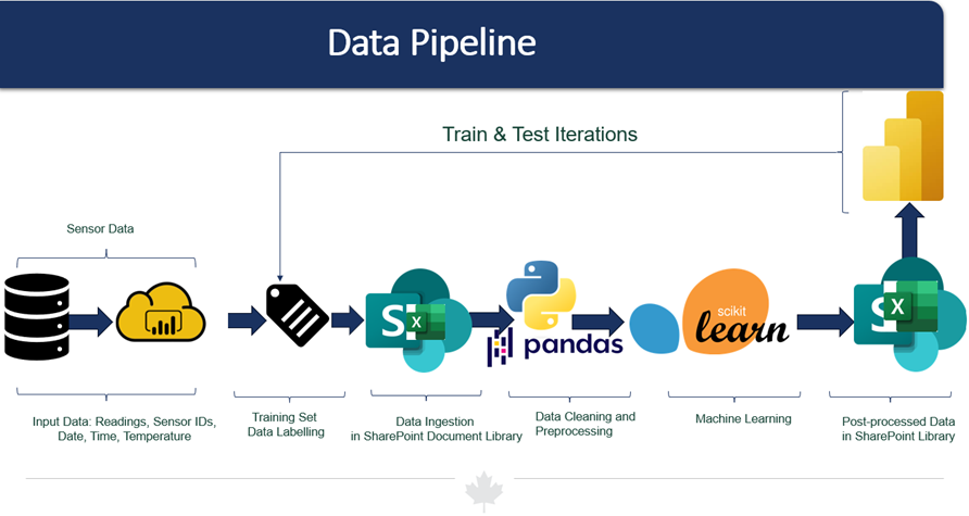
Description - Figure 1 : Data Pipeline
Figure 1 shows an image that illustrates the data pipeline for the project. It starts with input data, which includes Sensor readings, sensor IDs, date, time, and temperature. This data is ingested into a SharePoint Document Library. The next step in the pipeline is data cleaning and preprocessing, followed by machine learning. In the final step, the post-processed data is stored back in the SharePoint Library. The training set involves data labeling and train and test iterations. The entire project uses sensor data.
Methods
The project uses a semi-supervised ML classification approach similar to techniques discussed in our literature review section. This technique uses a combination of labelled and unlabelled data where we partially label a training set and apply statistical parameters in the anomaly detection process as described in the following sections. The choice of the method was motivated by multiple factors related to ensuring control over training data, the types of anomalies, cost-effectiveness, replicability, and performance, among others. Authors such as Soule et al. (2005) and Rousseeuw & Hubert (2017) proposed robust methods for using statistical techniques in anomaly detection and demonstrated the combination of such techniques with existing machine learning approaches yields robust results while the use of ML alone can generally miss hard-to-detect anomaly types (Spanos et al., 2019; Jasra et al., 2022). This indeed proved to be true in this project: when we applied an unsupervised ML model during the exploration phase, we realized that only outliers, i.e. data that were significantly above or below the centres, were being flagged as anomalies. Yet, we needed a method that can capture the anomalies that are not easily detected.
To successfully implement the approach, we partially labelled a sample set and trained a ML model to flag those anomalies. Prior to running the supervised model, we start by prepopulating anomaly predictions in an unsupervised and rule-based approach with pre-defined parameters for standard deviations and time series window sizes described in the following sections. With a partially labelled training set, ML classification is applied, and we chose the Gradient Boosting algorithm summarized by equations (1) and (2) below:
(1)
(2)
Where:
- is the predicted binary data label for a normal or an abnormal sensor reading;
- is a set of predictors for time series data with sensor reading, date and time;
- is the function learned by the classifier from the training (labeled) data;
- is a constant initial value for the target prediction;
- is the number of boosting stages, also called “weak learners”;
- are coefficients also known as the learning rate;
- are the weak learners or the decision trees
The expression in (1) represent the model’s predicted output y for input features x where F is the aggregated function combining all individual weak learners. The expression in (2) illustrates how the model is built iteratively over K boosting rounds: starting with an initial constant, each subsequent iteration adds a scaled weak learner to progressively minimize the residual errors.
It is important to note that the Gradient Boosting algorithm usually outperforms other ensemble learner models (Ebrahimi et al., 2019) and, in some instances, authors have found a gradient boosted decision tree was superior by a large margin to some neural models (Qin et al., 2021). Prior to employing the semi-supervised approach through the Gradient Boosting algorithm, we tested an Isolation Forest model as a fully unsupervised anomaly detection technique. Results of the Isolation Forests method did not meet our expectations in terms of accuracy, which is not surprising in such cases with conditional anomalies as shown by Pang et al. (2021) cited above.
This approach allowed full control over training data and gave room to possibilities of finetuning multiple parameters including model parameters such as testing and training sizes, random states as well as statistical parameters for standard deviations and time series window sizes. Indeed, we defined anomaly types by existing formulas defined by bridge engineers and by labelling training sets manually using an iterative process. For example, we were able to isolate the following type of anomalies called flatlines that were not flagged by the alarm system because they remained within the predefined thresholds previously mentioned and that would be time-consuming and not practical to identify manually:
- Absolute flatline anomalies: when a sensor returns exactly the same reading four times consecutively with standard deviation equal to 0
- Consecutive but relative flatline anomalies: when a sensor returns 12 consecutive readings in a day with very little fluctuation set to absolute standard deviation value inferior or equal to 0.15
The use of this semi-supervised approach also ensured that our method could be applied to similar problems without the need to rewrite the algorithm, hence ensuring cost effectiveness and replicability. Finally, the choice of this method was also motivated by the well documented compute efficiencies and performances for supervised machine learning models (Akinsola et al., 2019; Aboueata et al., 2019; Ma et al., 1999). It is worth noting that while the results were satisfactory, this approach had some limitations and challenges. In particular, the manual labelling of training data required significant efforts. Additionally, the combination of techniques, while allowing flexibility, had a risk for model overfitting which we are mitigating by carefully inspecting the predicted results with analysts’ knowledge.
Results and Discussion
In its first phase, the project led to the identification of 714,185 data readings flagged as anomalies. This represented roughly 4.6% of all sensor readings and fell in one of the following pre-determined categories:
- Anomalies caused by irregular fluctuations
- Anomalies related to the lack of normal fluctuations including absolute and relative flatlines
- Anomalies caused by readings being outside of the expected range for sensors
The proportion of data points identified as anomalies was over 4% larger than what a non-supervised Isolation Forest model had returned in an earlier exploration, confirming the conclusions by Pang et al. (2021) that more complex anomaly types require more advanced combination of methods for accurate detection. We also obtained an average internal accuracy score of 0.988 (or over 98%), which, while not an absolute indication of success, was a signal for the model’s performance.
Predictive Accuracy
During the proof-of-concept phase of this project, we computed an F1 score for model accuracy and obtained a score of 0.956 (96%) accuracy. The F1 score is the harmonic mean of a model's precision and recall scores and is often used to evaluate classification models (for example, see Silva et al., 2024; Zhang et al. 2015). In the following section, we report on the internal model accuracy computed using the cross-validation approach from the scikit-learn library. To avoid overfitting, we held on to a small sample of data as a test set and computed the accuracy score using the `train_test_split` method from scikit-learn. The method splits datasets into training and testing subsets for ML tasks. It has various parameters such as the ‘test_size’ and ‘train_size’ which determine, randomly or in controlled manner, the fraction of number of samples for the test and train set. This approach allows better control, especially in the cases of imbalanced training data.
This process is well documented by scikit-learn as shown in figure 2 below:
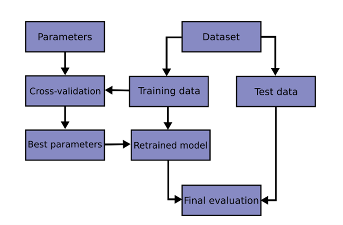
Figure 2: Splitting training and test set
Figure 2 shows an image that was taken from the Scikit-Learn Library to visually represents the process of dividing a dataset into training sets and test sets. The training set is used to train a machine learning model, while the test set is used to evaluate the model's performance. The image displays a diagram showing how the data is split, with arrows indicating the separation between the various elements of the train-test split process. Those elements are linked by arrows as follows: parameters, cross-validation, Best parameters, Dataset, Training data, Retrained model, Test data and Final Evaluation.
Table 1 below shows accuracy scores obtained for a sample of 9 sensors out of 44 sensors in the scope of the first phase of the project. This score is calculated by dividing the number of correct predictions by the number of total predictions and thus allows comparison of the predicted values with the actual values. The score was computed using the y_val_split, y_val_pred methods from the sklearn.metrics sub-library. It is worth noting that the exercise of partially labelling training data was done on a full cycle of the sensor readings, covering a sample year. This helped overcome the problem of imbalanced training set and resulted in comparable shares of anomalies in training data and anomalies identified.
| Sensor ID | Accuracy score |
|---|---|
| Sensor ID 1 | 0.998463902 |
| Sensor ID 2 | 0.998932764 |
| Sensor ID 3 | 0.990174672 |
| Sensor ID 4 | 0.98579235 |
| Sensor ID 5 | 0.99592668 |
| Sensor ID 6 | 0.994401679 |
| Sensor ID 7 | 0.998294486 |
| Sensor ID 8 | 0.998385361 |
| Sensor ID 9 | 0.99452954 |
While this score served as a good benchmark, it is worth noting that because of the specificity of anomalies being detected, more accuracy scoring metrics are being researched to ensure the best representation of the model’s performance.
Using the results: From Machine Learning to Business Value
The predicted anomalies need to be consumable to the bridge engineers so they can action on the insights produced by the ML model. The solution was to visualize the output in a simple and easy dashboard that summarizes the findings while providing enough information that can inform decision-making. We used Microsoft’s Power BI to produce a simplistic visualization that contain the following information:
- Anomaly percentage by day using a stacked column chart, which can be drilled up to anomaly percentage by month
- The sensor readings using a line chart and differentiating between normal readings and anomalies
- A table with the detailed results provided by the algorithm for the selected sensor and year/month.
- The performance indicator for the selected sensor for the selected time range, which is the percentage of the number of normal readings over the total number of readings
- The share of normal sensor readings vs anomalies (donut chart) and a filter for comparison
Anomaly percentage by day using a stacked column chart, which can be drilled up to anomaly percentage by month
This type of dashboard is used to determined how well a specific sensor is performing and if it needs calibration, repair, or replacement. It provides limited visibility on the behaviour of the structure that the sensor is monitoring.
A snapshot of the dashboard showing the above is provided in Figure 3 below.
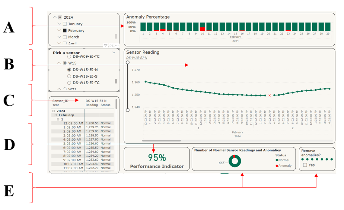
Figure 3: Results Visualization (1)
Figure 3 is an image that shows a visual representation of the results from the project. The image is divided into several sections each labelled with letters A through F. Section A displays a line chart with multiple lines representing different sensors. The lines show the sensor readings over time, with anomalies removed from the visual. Section B shows the correlation between the sensor readings and the inverse of temperature, and how temperature fluctuations impact the sensor data. Section C shows the offsets between the displacement lines removed so they could overlap to provide a clearer comparison of the sensor data. Section D presents the monthly averages of the sensor readings and gives an overview of the data trends over time. Section E includes performance indicators for all the selected sensors and shows the accuracy and reliability of the sensor readings. Section F provides additional details and insights about the sensor data and the detected anomalies.
We also ensured the results can be visualized together for all sensors which allowed comparison and readability. The three figures below show the steps performed in order to attain this comparison and readability.
Unlike the previous dashboard, this type of dashboard, once anomalies such as noise and outliers are removed, allows for better visibility of the trends and the behaviour of the structures that the sensors are monitoring, as opposed to the behaviour of the sensors themselves.
Figure 4 shows the initial raw data of multiple sensors on the same graph, averaged monthly to show the results over extended periods of time (i.e. trend evaluation), along with temperature, which is distinguished by being dashed, as temperature is the main influencing reading predictor.
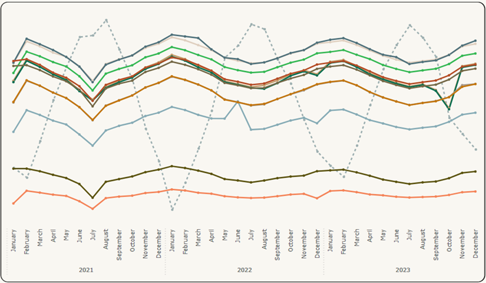
Figure 4: Results Visualization (2) – Initial Data
Figure 4 is an image with a multiple-lines graph showing the trends and distribution of the initial data. The lines have different colors, each representing a different sensor over time. A dotted line shows temperature readings. The time is displayed by year and by month starting January 2021 and ending in December 2023. The lines representing sensors are scattered throughout the time axis.
In Figure 5, the offsets between the sensor data lines are removed to ensure overlapping, and temperature is inverted so that it can also follow the upward and downward trend of the sensor data lines.
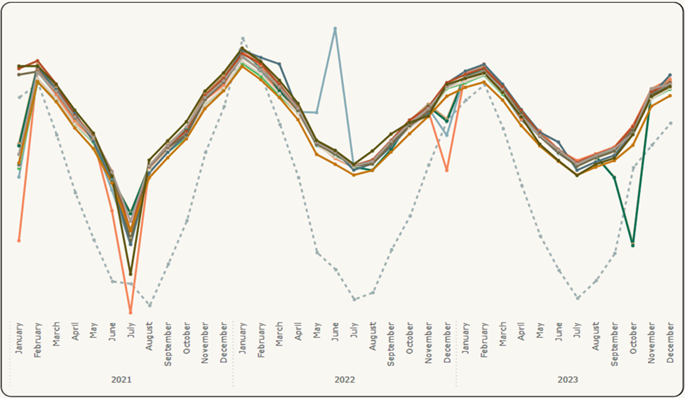
Figure 5: Results Visualization (2) – Initial Data with Improved Visuals
Figure 5 is an image that has a multiple-lines graph showing the trends and distribution of the initial data with improvement. The lines have different colors, each representing a different sensor over time. A dotted line shows temperature readings. The time is displayed by year and by month starting January 2021 and ending in December 2023. The lines representing sensors are less scattered throughout the time axis compared to the previous image with initial results.
Finally, Figure 6. displays the final results with the removal of anomalies detected by our model. Once more, the overlap of temperature with the sensor data allows to qualitatively evaluate the behaviour of the structures at a glance.
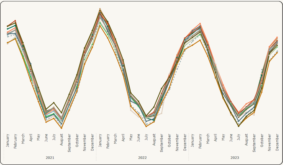
Figure 6: Results Visualization (2) – Final Results
Figure 6 is an image that has a multiple-lines graph showing the trends and distribution of the initial data with improvement. The lines have different colors, each representing a different sensor over time. A dotted line shows temperature readings. The time is displayed by year and by month starting January 2021 and ending in December 2023. The lines representing sensors are not scattered but show similar trends throughout the time axis compared to the previous two images.
The results obtained in this project have demonstrated the potential for using ML approaches to improve the anomaly detection exercise and to ensure a more efficient and accurate monitoring of sensor data. Indeed, the project has contributed to understanding historical data on bridge sensors and provided insights on the overall performance of the sensors. Moreover, the results assisted the Bridge Team in evaluating the performance of sensors, ultimately flagging a number of them for further analysis. Once the sensors are investigated and their functionality confirmed, the now noise-less data allows for a better appreciation of the behaviour of the structure, its performance trends, and its structural health over time.
Our approach has proven to have the potential to assist during the bridge operation, maintenance, and rehabilitation phase by helping to contribute towards early detection and inspection planning for infrastructure. Additionally, by exploring and manipulating historical data, the project has contributed to the overall objective of bridge health monitoring by checking data quality and reliability. The data quality checks that come with anomaly detection will help improve the accuracy of historical bridge SHMS data and facilitate the planning and management of future work. The control over anomaly types reduces the occurrence of false alarms while opening avenue for detailed inspections and checks. The resulting visualization will also be handy for the technical team and will provide insights on the performance of the sensors, as well as potential structural issues.
Conclusion and Next Steps
This project sought to leverage advanced techniques combining semi-supervised ML and statistical approaches for anomaly detection. As demonstrated in the literature section, anomaly detection is a complex problem that requires expertise and is usually well achieved by combining a host of methods. Indeed, we have shown that the exercise has the potential to flag sensor data anomalies in a controlled and replicable manner. In the next phases of the project, a multi-class model is being researched to ensure that not only anomalies are detected but they are also labelled and clustered into specific anomaly types. This granular approach will improve diagnostic clarity and help engineers to better understand sensor anomaly causes and ultimately support bridge maintenance.
It is worth noting, in this concluding paragraph, that with the advent of Generative AI (GenAI), future research should explore its potential for anomaly detection. GenAI has the ability to learn patterns and distributions of normal data and therefore could, if provided with examples, identify deviations that may signify anomalous data readings. Additionally, by training models like Generative Adversarial Networks (GANs) on large datasets, researchers can generate realistic representations of typical behavior and enhance anomaly detection exercises. The use of GenAI was outside of the scope of this project.
Subscribe to the Data Science Network for the Federal Public Service newsletter to keep up with the latest data science news.
References
- Aboueata, N., Alrasbi, S., Erbad, A., Kassler, A., & Bhamare, D. (2019). Supervised Machine Learning Techniques for Efficient Network Intrusion Detection. 2019 28th International Conference on Computer Communication and Networks (ICCCN), 1–8. https://doi.org/10.1109/ICCCN.2019.8847179
- A insola, J., Awodele, O., Kuyoro, S., & Kasali, F. (2019). Performance Evaluation of Supervised Machine Learning Algorithms Using Multi-Criteria Decision Making Techniques. https://www.researchgate.net/publication/343833347
- Chandola, V., Banerjee, A., & Kumar, V. (2009). Anomaly detection: A survey. ACM Computing Surveys, 41(3), 1–58. https://doi.org/10.1145/1541880.1541882
- Ebrahimi, M., Mohammadi-Dehcheshmeh, M., Ebrahimie, E., & Petrovski, K. R. (2019). Comprehensive analysis of machine learning models for prediction of sub-clinical mastitis: Deep Learning and Gradient-Boosted Trees outperform other models. Computers in Biology and Medicine, 114, 103456. https://doi.org/10.1016/j.compbiomed.2019.103456
- Jasra, S. K., Valentino, G., Muscat, A., & Camilleri, R. (2022). Hybrid Machine Learning–Statistical Method for Anomaly Detection in Flight Data. Applied Sciences, 12(20), 10261. https://doi.org/10.3390/app122010261
- Nassif, A. B., Talib, M. A., Nasir, Q., & Dakalbab, F. M. (2021). Machine Learning for Anomaly Detection: A Systematic Review. IEEE Access, 9, 78658–78700. https://doi.org/10.1109/ACCESS.2021.3083060
- Pang, G., Shen, C., Cao, L., & Hengel, A. V. D. (2021). Deep Learning for Anomaly Detection: A Review. ACM Computing Surveys, 54(2), 1–38. https://doi.org/10.1145/3439950
- Qin, Z., Yan, L., Zhuang, H., Pasumarthi, R. K., Wang, X., Bendersky, M., & Najork, M. (2021). Are Neural Rankers still Outperformed by Gradient Boosted Decision Trees? International Conference on Learning Representations (ICLR). https://research.google/pubs/are-neural-rankers-still-outperformed-by-gradient-boosted-decision-trees/
- Rousseeuw, P. J., & Hubert, M. (2018). Anomaly detection by robust statistics. WIREs Data Mining and Knowledge Discovery, 8(2), e1236. https://doi.org/10.1002/widm.1236
- Scikit Learn. (2024). User Guide - 3.1. Cross-validation: evaluating estimator performance. https://scikit-learn.org/stable/modules/cross_validation.html
- Sheng Ma, & Chuanyi Ji. (1999). Performance and efficiency: recent advances in supervised learning. Proceedings of the IEEE, 87(9), 1519–1535. https://doi.org/10.1109/5.784228
- Silva, P., Baye, G., Broggi, A., Bastian, N. D., Kul, G., & Fiondella, L. (2024). Predicting F1-Scores of Classifiers in Network Intrusion Detection Systems. 2024 33rd International Conference on Computer Communications and Networks (ICCCN), 1–6. https://doi.org/10.1109/ICCCN61486.2024.10637544
- Soule, A., Salamatian, K., & Taft, N. (2005). Combining Filtering and Statistical Methods for Anomaly Detection. Proceedings of the 5th ACM SIGCOMM Conference on Internet Measurement. https://www.usenix.org/legacy/events/imc05/tech/full_papers/soule/soule.pdf
- Spanos, G., Giannoutakis, K. M., Votis, K., & Tzovaras, D. (2019). Combining Statistical and Machine Learning Techniques in IoT Anomaly Detection for Smart Homes. 2019 IEEE 24th International Workshop on Computer Aided Modeling and Design of Communication Links and Networks (CAMAD), 1–6. https://doi.org/10.1109/CAMAD.2019.8858490
- Zhang, D., Wang, J., & Zhao, X. (2015). Estimating the Uncertainty of Average F1 Scores. Proceedings of the 2015 International Conference on The Theory of Information Retrieval, 317–320. https://doi.org/10.1145/2808194.2809488.